Random Search Methods
Random Search Methods. Simulated Annealing Tabu Search Genetic Algorithms Job scheduling problem Branch-and-bound Beam search. Simulated Annealing (SA). Notation S 0 is the best solution found so far S k is the current solution G(S k ) it the performance of a solution Note that.

Random Search Methods
E N D
Presentation Transcript
Random Search Methods • Simulated Annealing • Tabu Search • Genetic Algorithms • Job scheduling problem • Branch-and-bound • Beam search
Simulated Annealing (SA) • Notation • S0 is the best solution found so far • Sk is the current solution • G(Sk) it the performance of a solution • Note that Aspiration Criterion
Acceptance Criterion • Let Sc be the candidate solution • If G(Sc) < G(Sk) accept Sc and let • If G(Sc)G(Sk) move to Sc with probability Always 0 Temperature > 0
Cooling Schedule • The temperature should satisfy • Normally we let but we sometimes stop when some predetermined final temperature is reached • If temperature is decreased slowly convergence is guaranteed
SA Algorithm Step 1: Set k = 1 and select the initial temperature b1. Select an initial solution S1 and set S0 = S1. Step 2: Select a candidate solution Sc from N(Sk). If G(S0) < G(Sc) < G(Sk), set Sk+1 = Sc and go to Step 3. If G(Sc) < G(S0), set S0 = Sk+1 = Sc and go to Step 3. If G(Sc) < G(S0), generate Uk Uniform(0,1); If Uk P(Sk, Sc), set Sk+1 = Sc; otherwise set Sk+1 = Sk; go to Step 3. Step 3: Select bk+1 bk. Let k=k+1. If k=N STOP; otherwise go to Step 2.
Discussion • SA has been applied successfully to many industry problems • Allows us to escape local optima • Performance depends on • Construction of neighborhood • Cooling schedule
Tabu Search • Similar to SA but uses a deterministic acceptance/rejection criterion • Maintain a tabu list of solution changes • A move made entered at top of tabu list • Fixed length (5-9) • Neighbors restricted to solutions not requiring a tabu move
Tabu List • Rational • Avoid returning to a local optimum • Disadvantage • A tabu move could lead to a better schedule • Length of list • Too short cycling (“stuck”) • Too long search too constrained
Tabu Search Algorithm Step 1: Set k = 1. Select an initial solution S1 and set S0 = S1. Step 2: Select a candidate solution Sc from N(Sk). If Sk Sc on tabu list set Sk+1 = Sk and go to Step 3. Enter Sc Sk on tabu list. Push all the other entries down (and delete the last one). If G(Sc) < G(S0), set S0= Sc. Go to Step 3. Step 3: Select bk+1 bk. Let k=k+1. If k=N STOP; otherwise go to Step 2.
Scheduling Problem • Allocate scarce resources to tasks • Combinatorial optimization problem Maximize profit Subject to constraints • Mathematical techniques and heuristics
Decision Variables • Three basic types of solutions: • A sequence: a permutation of the jobs • A schedule: allocation of the jobs in a more complicated setting of the environment • A scheduling policy: determines the next job given the current state of the system
Objectives and Performance Measures • Throughput (TP) and makespan (Cmax) • Due date related objectives • Work-in-process (WIP), lead time (response time), finished inventory • Others
Initialization • Tabu list empty L={} • Initial schedule S1 = (2,1,4,3) 20 - 4 = 16 10 - 2 = 8 Deadlines 37 - 1 = 36 24 - 12 = 12 0 10 20 30 40
Neighborhood • Define the neighborhood as all schedules obtain by adjacent pairwise interchanges • The neighbors of S1 = (2,1,4,3) are (1,2,4,3) (2,4,1,3) (2,1,3,4) • Objective values are: 480, 436, 652 Select the best non-tabu schedule
Second Iteration • Let S0 =S2 = (2,4,1,3). G(S0)=436. • Let L = {(1,4)} • New neighborhood
Third Iteration • Let S3 = (4,2,1,3), S0 = (2,4,1,3). • Let L = {(2,4),(1,4)} • New neighborhood Tabu!
Fourth Iteration • Let S4 = (4,1,2,3), S0 = (2,4,1,3). • Let L = {(1,2),(2,4)} • New neighborhood
Fifth Iteration • Let S5 = (1,4,2,3), S0 = (1,4,2,3). • Let L = {(1,4),(1,2)} • This turns out to be the optimal schedule • Tabu search still continues • Notes: • Optimal schedule only found via tabu list • We never know if we have found the optimum!
Genetic Algorithms • Schedules are individuals that form populations • Each individual has associated fitness • Fit individuals reproduce and have children in the next generation • Very fit individuals survive into the next generation • Some individuals mutate
Total Weighted Tardiness Single Machine Example • First Generation Initial population selected randomly
Mutation Operator Fittest Individual Reproduction via mutation (4,3,1,2)
Cross-Over Operator Fittest Individuals (4,1,3,2) (2,1,3,4) (2,1,3,2) (4,1,3,4) Reproduction via cross-over Infeasible!
Representing Schedules • When using GA we often represent individuals using binary strings (0 1 1 0 1 0 1 0 1 0 1 0 0 ) (1 0 0 1 1 0 1 0 1 0 1 1 1 ) (0 1 1 0 1 0 1 0 1 0 1 1 1 )
Discussion • Genetic algorithms have been used very successfully • Advantages: • Very generic • Easily programmed • Disadvantages: • A method that exploits special structure is usually faster (if it exists)
Branch and Bound • Enumerative method • Guarantees finding the best schedule • Basic idea: • Look at a set of schedules • Develop a bound on the performance • Discard (fathom) if bound worse than best schedule found before
Classic Results • The EDD rule is optimal for • If jobs have different release dates, which we denote then the problem is NP-Hard • What makes it so much more difficult?
EDD 1 2 3 0 5 10 15 Can we improve?
Delay Schedule Add a delay 1 3 2 0 5 10 15 What makes this problem hard is that the optimal schedule is not necessarily a non-delay schedule
Final Classic Result • The preemptive EDD rule is optimal for the preemptive (prmp) version of the problem • Note that in the previous example, the preemptive EDD rule gives us the optimal schedule
Branch and Bound • The problem cannot be solved using a simple dispatching rule so we will try to solve it using branch and bound • To develop a branch and bound procedure: • Determine how to branch • Determine how to bound
Branching (•,•,•,•) (1,•,•,•) (2,•,•,•) (3,•,•,•) (4,•,•,•)
Branching (•,•,•,•) (1,•,•,•) (2,•,•,•) (3,•,•,•) (4,•,•,•) Discard immediately because
Branching (•,•,•,•) (1,•,•,•) (2,•,•,•) (3,•,•,•) (4,•,•,•) Need to develop lower bounds on these nodes and do further branching.
Bounding (in general) • Typical way to develop bounds is to relax the original problem to an easily solvable problem • Three cases: • If there is no solution to the relaxed problem there is no solution to the original problem • If the optimal solution to the relaxed problem is feasible for the original problem then it is also optimal for the original problem • If the optimal solution to the relaxed problem is not feasible for the original problem it provides a bound on its performance
Relaxing the Problem • The problem is a relaxation to the problem • Not allowing preemption is a constraint in the original problem but not the relaxed problem • We know how to solve the relaxed problem (preemptive EDD rule)
Bounding • Preemptive EDD rule optimal for the preemptive version of the problem • Thus, solution obtained is a lower bound on the maximum delay • If preemptive EDD results in a non-preemptive schedule all nodes with higher lower bounds can be discarded.
Lower Bounds • Start with (1,•,•,•): • Job with EDD is Job 4 but • Second earliest due date is for Job 3 Job 1 Job 2 Job 3 Job 4 0 10 20
Branching (•,•,•,•) (1,•,•,•) (2,•,•,•) (3,•,•,•) (4,•,•,•) (1,2,•,•) (1,3,•,•) (1,3,4,2)
Beam Search • Branch and Bound: • Considers every node • Guarantees optimum • Usually too slow • Beam search • Considers only most promising nodes • (beam width) • Does not guarantee convergence • Much faster
Branching (Beam width = 2) (•,•,•,•) (1,•,•,•) (2,•,•,•) (3,•,•,•) (4,•,•,•) ATC Rule (1,4,2,3) (2,4,1,3) (3,4,1,2) (4,1,2,3) 408 436 814 440
Beam Search (•,•,•,•) (1,•,•,•) (2,•,•,•) (3,•,•,•) (4,•,•,•) (1,2,•,•) (1,3,•,•) (1,4,•,•) (2,1,•,•) (2,3,•,•) (2,4,•,•) (1,4,2,3) (1,4,3,2) (2,4,1,3) (2,4,3,1)
Discussion • Implementation tradeoff: • Careful evaluation of nodes (accuracy) • Crude evaluation of nodes (speed) • Two-stage procedure • Filtering • crude evaluation • filter width > beam width • Careful evaluation of remaining nodes