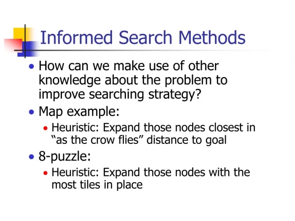
Informed Search Methods
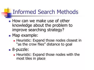
How can we improve searching strategy by using intelligence? Map example: Heuristic: Expand those nodes closest in “as the crow flies” distance to goal 8-puzzle: Heuristic: Expand those nodes with the most tiles in place Intelligence lies in choice of heuristic. Informed Search Methods.

Informed Search Methods
E N D
Presentation Transcript
How can we improve searching strategy by using intelligence? Map example: Heuristic: Expand those nodes closest in “as the crow flies” distance to goal 8-puzzle: Heuristic: Expand those nodes with the most tiles in place Intelligence lies in choice of heuristic Informed Search Methods
Best-First Search • Create evaluation function f(n) which returns estimated “value” of expanding node • Example: Greedy best-first search • “Greedy”: estimate cost of cheapest path from node n to goal • h(n) = “as the crow flies distance” • f(n) = h(n)
GreedyBest-First Search h(n)=366 A h(n)=374 h(n)=253 h(n)=329 T Z S A O F R h(n)=178 h(n)=193 h(n)=366 h(n)=380 S B h(n)=253 h(n)=0
Greedy Best-First Search • Expand the node with smallest h • Why is it called greedy? • Expands node that appears closest to goal • Similar to depth-first search • Follows single path all the way to goal, backs up when dead end • Worst case time: • O(bm), m = depth of search space • Worst case memory: • O(bm), needs to store all nodes in memory to see which one to expand next
Greedy Best-First Search • Complete and/or optimal? • No – same problems as depth first search • Can get lost down an incorrect path • How can you (help) to prevent it from getting lost? • Look at shortest total path, not just path to goal
A* search (another Best-First Search) • Greedy best-first search minimizes • h(n) = estimated cost to goal • Uniform cost search minimizes • g(n) = cost to node n • Example of each on map • A* search minimizes • f(n) = g(n) + h(n) • f(n) = best estimate of cost for complete solution through n
A* search • Under certain conditions: • Complete • Terminates to produce best solution • Conditions • (assuming we don’t throw away duplicates) • h(n) must never overestimate cost to goal • admissible heuristic • “optimistic” • “Crow flies” heuristic is admissible
A*Search f(n) = 366 A f(n) = 449 f(n) = 393 f(n) = 447 T Z S A O F R f(n) = 417 f(n) = 413 f(n) = 646 f(n) = 526 C P S f(n) = 526 f(n) = 415 f(n) = 553
A*Search A O F R f(n) = 417 f(n) = 413 f(n) = 646 f(n) = 526 C R P C B S f(n) = 526 f(n) = 607 f(n) = 415 f(n) = 615 f(n) = 553 f(n) = 418
A*Search f(n) = 366 A f(n) = 449 f(n) = 393 f(n) = 447 T Z S A O F R f(n) = 417 f(n) = 413 f(n) = 646 f(n) = 526 S B f(n) = 591 f(n) = 450
A* terminates with optimal solution • Stop A* when you try to expand a goal state. • This the best solution you can find. • How do we know that we’re done when the next state to expand is a goal? • A* always expands node with smallest f • At a goal state, f is exact. • Since heuristic is admissible, f is an underestimate at any non-goal state. • If there is a better goal state available, with a smaller f, there must be a node on graph with smaller f than that – so you would be expanding that instead!
More about A* • Completeness • A* expands nodes in order of increasing f • Must find goal state unless • infinitely many nodes with f(n) < f* • infinite branching factor OR • finite path cost with infinite nodes on it • Complexity • Time: Depends on h, can be exponential • Memory: O(bm), stores all nodes
Valuing heuristics • Example: 8-puzzle • h1 = # of tiles in wrong position • h2 = sum of distances of tiles from goal position (1-norm, also known as Manhattan distance) • Which heuristic is better for A*?
Which heuristic is better? • h2(n) >= h1(n) for any n • h2 dominates h1 • A* will generally expand fewer nodes with h2 than with h1 • All nodes with f(n) < C* (cost to best solution) are expanded. • Since h2 >= h1, any node that A* expands with h2 would also be expanded with h1 • But A* may be able to avoid expanding some nodes with h2 (larger than C*) • (Exception where you might expand a state with h2 but not with h1: if f(n) = C*). • Better to use larger heuristic (if not overestimate)
Inventing heuristics • h1 and h2 are exact path lengths for simpler problems • h1 = path length if you could transport each tile to right position • h2 = path length if you could just move each tile to right position, irrelevant of blank space • Relaxed problem: less restrictive problem than original • Can generate heuristics as exact cost estimates to relaxed problems
Memory Bounded Search • Can A* be improved to use less memory? • Iterative deepening A* search (IDA*) • Each iteration is a depth-first search, just like regular iterative deepening • Each iteration is not an A* iteration: otherwise, still O(bm) memory • Use limit on cost (f), instead of depth limit as in regular iterative deepening
IDA*Search f-Cost limit = 366 f(n) = 366 A f(n) = 449 f(n) = 393 f(n) = 447 T Z S
IDA*Search f-Cost limit = 393 f(n) = 366 A f(n) = 449 f(n) = 393 f(n) = 447 T Z S A O F R f(n) = 417 f(n) = 415 f(n) = 646 f(n) = 526
IDA* Analysis • Time complexity • If cost value for each node is distinct, only adds one state per iteration • BAD! • Can improve by increasing cost limit by a fixed amount each time • If only a few choices (like 8-puzzle) for cost, works really well • Memory complexity • Approximately O(bd) (like depth-first) • Completeness and optimality same as A*
Simplified Memory-Bounded A* (SMA*) • Uses all available memory • Basic idea: • Do A* until you run out of memory • Throw away node with highest f cost • Store f-cost in ancestor node • Expand node again if all other nodes in memory are worse
SMA* Example: Memory of size 3 A f = 12
SMA* Example: Memory of size 3 A f = 12 B f = 15 Expand to the left
SMA* Example: Memory of size 3 A f = 12 B f = 15 C f = 13 Expand node A, since f smaller
SMA* Example: Memory of size 3 A f = 12 forgotten f = 15 C f = 13 D f = 18 Expand node C, since f smaller
SMA* Example: Memory of size 3 A f = 12 forgotten f = 15 C f = 13 forgotten f = infinity E f = 24 Node D not a solution, no more memory: so expand C again
SMA* Example: Memory of size 3 A f = 12 B f = 15 C f = 13 Forgottenf = 24 (right) Re-expand A; record new f for C
SMA* Example: Memory of size 3 A f = 12 forgotten = 24 B f = 15 F f = 25 Expand left B: not a solution, so useless
SMA* Example: Memory of size 3 A f = 12 Forgotten f = 24 B f = 15 forgotten f = inf G f = 20 Expand right B: find solution
SMA* Properties • Complete if can store at least one solution path in memory • Finds best solution (and recognizes it) if path can be stored in memory • Otherwise, finds best that can fit in memory