Blind and Informed Search Methods
Blind and Informed Search Methods. Filename: eie426-search-methods-0809.ppt. Contents:. Problem types Problem formulation Example problems Basic search algorithms: - breadth-first search - depth-first search Best-first search - greedy search - A* search. Example: Romania.

Blind and Informed Search Methods
E N D
Presentation Transcript
Blind and Informed Search Methods Filename: eie426-search-methods-0809.ppt EIE426-AICV
Contents: • Problem types • Problem formulation • Example problems • Basic search algorithms: - breadth-first search - depth-first search • Best-first search - greedy search - A* search EIE426-AICV
Example: Romania On holiday in Romania; currently in Arad. Flight leaves tomorrow for Bucharest. Formulate goal: be in Bucharest Formulate problem: states: various cities actions: flight between cities Find solution: sequence of cities, e.g., Arad, Sibiu, Fagaras, Bucharest EIE426-AICV
Example: Romania (cont.) EIE426-AICV
Selecting a state space Real world is absurdly complex =〉state space must be abstracted for problem solving (Abstract) state = set of real states (Abstract) action = complex combination of real actions e.g., “Arad => Zerind'' represents a complex set of possible routes, detours, rest stops, etc. For guaranteed realizability, any real state “in Arad” must get to some real state “in Zerind” (Abstract) solution = set of real paths that are solutions in the real world Each abstract action should be “easier” than the original problem! EIE426-AICV
State Space Representation of Problems • Nodes (N): partial solution states • Arcs (A): the steps in a problem-solving process. • Initial States (one or more) (S): the given information in a problem instance, form the root of the graph • Goal States (GD): the solutions to a problem instance • State Space Search: finding a solution path from the start state to a goal A state space is represented by a four-tuple [N, A, S, GD]. EIE426-AICV
Example: The 8-puzzle states: integer locations of tiles (ignore intermediate positions) actions: move blank left, right, up, down goal test: = goal state (given) path cost: 1 per move EIE426-AICV
Example: The Traveling Salesperson • Suppose a salesperson has N cities to visit and must return home. The goal of the problem is to find the shortest path for the salesperson to travel, visiting each city, and then returning to the starting city. • Nodes: cities • Arcs: labeled with a weight indicating the cost of traveling • Complexity: (N-1)! EIE426-AICV
Example: The Traveling Salesperson (cont.) EIE426-AICV
Example: Tic-Tac-Toe • The start state: an empty board • The goal description: three Xs or three Os in a row, column, or diagonal • A directed acyclic graph (DAG) • Arc: a legal move (placing an X or O in an unused location • The complexity: 9!=362,880 paths EIE426-AICV
Tree search algorithms Basic idea: offline, simulated exploration of state space by generating successors of already-explored states (also known as expanding states) EIE426-AICV
Tree search example EIE426-AICV
Implementation: states vs. nodes A state is a (representation of) a physical configuration A node is a data structure constituting part of a search tree includes parent, children, depth, path cost g(x) States do not have parents, children, depth, or path cost! The Expand function creates new nodes, filling in the various fields and using the SuccessorFn of the problem to create the corresponding states. EIE426-AICV
Implementation: general tree search EIE426-AICV
Search strategies A strategy is defined by picking the order of node expansion Strategies are evaluated along the following dimensions: Completeness -- does it always find a solution if one exists? Time complexity -- number of nodes generated/expanded Space complexity -- maximum number of nodes in memory Optimality -- does it always find a least-cost solution? Time and space complexity are measured in terms of b --- maximum branching factor of the search tree d --- depth of the least-cost solution m --- maximum depth of the state space (may be ) EIE426-AICV
Uninformed search strategies Uninformed strategies use only the information available in the problem definition Breadth-first search Depth-first search etc. EIE426-AICV
4 4 B C A 3 5 5 S G 4 3 2 4 F D E A Search Tree Two costs: finding a path and traversing the path. S G EIE426-AICV
4 4 B C A 3 5 5 S G 4 3 2 4 F D E Search Trees (cont.) b = 2 d = 0, 1, …,6 m = 6 From the left to the right: alphabetical order EIE426-AICV
Breadth-First Search Expand shallowest unexpanded node Implementation: fringe is an FIFO queue, i.e., new successors go at end EIE426-AICV
B C A S G F D E Breadth-First Search (cont.) Expand shallowest unexpanded node Implementation: fringe is a FIFO queue, i.e., new successors go at end EIE426-AICV
Properties of breadth-first search Complete? Yes (if b is finite) Time? 1+b+b^2+b^3+…+b^d + b(b^d-1)= O(b^(d+1)), i.e., exponential in d Space? O(b^(d+1)) (keeps every node in memory) Optimal? Yes (if cost = 1 per step); not optimal in general Space is the big problem; can easily generate nodes at 10 MB/sec so 24 hrs = 860 GB. EIE426-AICV
Depth-First Search Expand deepest unexpanded node Implementation: fringe = LIFO queue, i.e., put successors at front EIE426-AICV
B C A S G F D E Depth-First Search (cont.) EIE426-AICV
Properties of depth-first search Complete? No: fails in infinite-depth spaces, spaces with loops Modify to avoid repeated states along path => complete in finite spaces Time? O(bm): terrible if m is much larger than d but if solutions are dense, may be much faster than breadth-first Space? O(bm), i.e., linear space! Optimal? No EIE426-AICV
A comparison between depth-first search and breadth-first search Advantages of Depth-First Search • It requires less memory. • By chance, it may find a solution without examining much of the search space at all. Advantages of Breadth-First Search • It will not get trapped exploring a blind alley. • If there are multiple solutions, then a minimal solution will be found. EIE426-AICV
Summary Problem formulation usually requires abstracting away real-world details to define a state space that can feasibly be explored Variety of uninformed search strategies EIE426-AICV
Best-first search Idea: use an evaluation function for each node -- estimation of “desirability” =〉 Expand most desirable unexpanded node Implementation: fringe is a queue sorted in decreasing order of desirability Special cases: • greedy search • A* search EIE426-AICV
Romania with step costs in km EIE426-AICV
Greedy search Evaluation function h(n) (heuristic) = estimate of cost from n to the closest goal E.g., hSLD(n) = straight-line distance from n to Bucharest Greedy search expands the node that appears to be closest to goal EIE426-AICV
Greedy search example EIE426-AICV
Properties of greedy search Complete? No -- can get stuck in loops, e.g., Iasi Neamt Iasi Neamt Complete in finite space with repeated-state checking Time? O(b^m), but a good heuristic can give dramatic improvement Space? O(b^m)---keeps all nodes in memory Optimal? No EIE426-AICV
A* search Idea: avoid expanding paths that are already expensive Evaluation function f(n) = g(n) + h(n) g(n) = cost so far to reach n h(n) = estimated cost to goal from n f(n) = estimated total cost of path through n to goal A* search uses an admissible heuristic i.e., h(n) h*(n) where h*(n) is the true cost from n. (Also require h(n) 0, so h(G)=0 for any goal G.) E.g., hSLD(n) never overestimates the actual road distance Theorem: A* search is optimal. EIE426-AICV
A* search example EIE426-AICV
Optimality of A* (standard proof) Suppose some suboptimal goal G2 has been generated and is in the queue. Let n be an unexpanded node on a shortest path to an optimal goal G1. f(G2) = g(G2) since h(G2) = 0 > g(G1) since G2 is suboptimal f(n) since h is admissible Since f(G2) > f(n), A* will never select G2 for expansion EIE426-AICV
Properties of A* Complete? Yes, unless there are infinitely many nodes with f f(G) Time? Depends on the heuristic. In the worse case, exponential in the length of the solution. Space? Keeps all nodes in memory Optimal? Yes EIE426-AICV
h Overestimates h* Step cost = 1 Miss this solution! The search may miss the optimal solution if there is any overestimate h. EIE426-AICV
Admissible Heuristics E.g., for the 8-puzzle: h1(n) = number of misplaced tiles h2(n) = total Manhattan distance (i.e., no. of squares from desired location of each tile) h1(S) = 7 h2(S) = 4+0+3+3+1+0+2+1 = 14 EIE426-AICV
Dominance If h2(n) h1(n) for all n (both admissible) then h2 dominates h1 and is better for search Typical search costs: d=14 A*(h1) = 539 nodes A*(h2) = 113 nodes d=24 A*(h1) = 39,135 nodes A*(h2) = 1,641 nodes EIE426-AICV
Example: n-queens Put n queens on an n times n board with no two queens on the same row, column, or diagonal. Move a queen to reduce number of conflicts. EIE426-AICV
Example: Heuristics and A* Search for Solving the 8-Puzzle problem EIE426-AICV
2 1 3 8 4 7 5 6 2 x 2 = 4 EIE426-AICV
Heuristic: Sum of distances out of place EIE426-AICV
Part of the Search Family of Procedures EIE426-AICV
Search Alternatives from a Procedure Family • Depth-first search is good when unproductive partial paths are never too long. • Breadth-first search is good when the branching factor is never too large. • A* search is good when a good heuristic is available. Search Animations EIE426-AICV