Map projections
Map projections . The dilemma. Maps are flat, but the Earth is not!. Producing a perfect map is like peeling an orange and flattening the peel without distorting a map drawn on its surface. For example:. The Public Land Survey System.

Map projections
E N D
Presentation Transcript
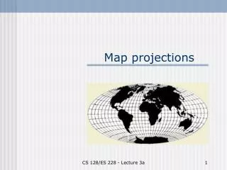
Map projections CS 128/ES 228 - Lecture 3a
The dilemma Maps are flat, but the Earth is not! Producing a perfect map is like peeling an orange and flattening the peel without distorting a map drawn on its surface. CS 128/ES 228 - Lecture 3a
For example: The Public Land Survey System • As surveyors worked north along a central meridian, the sides of the sections they were creating converged • To keep the areas of each section ~ equal, they introduced “correction lines” every 24 miles CS 128/ES 228 - Lecture 3a
Like this Township Survey Kent County, MI 1885 http://en.wikipedia.org/wiki/Image:Kent-1885-twp-co.jpg CS 128/ES 228 - Lecture 3a
One very practical result The jog created by these “correction lines”, where the old north-south line abruptly stopped and a new one began 50 or 60 yards east or west, became a feature of the grid, and because back roads tend to follow surveyors’ lines, they present an interesting driving hazard today. After miles of straight gravel or blacktop, the sudden appearance of a correction line catches most drivers by surprise, and frantic tire marks show where vehicles have been thrown into hasty 90-dgree turns, followed by a second skid after a short stretch running west or east when the road head north again onto the new meridian.Andro Linklater. 2002. Measuring America. Walker & Co., NY. P. 162 CS 128/ES 228 - Lecture 3a
Geographical (spherical) coordinates Latitude & Longitude (“GCS” in ArcMap) • Both measured as angles from center of Earth • Reference planes: - Equator for latitude- Prime meridian for longitude CS 128/ES 228 - Lecture 3a
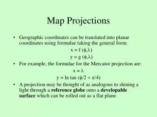
Lat/Long. are not Cartesian coordinates • They are angles measured from the center of Earth • They can’t be used (directly) to plot locations on a plane Understanding Map Projections. ESRI, 2000 (ArcGIS 8). P. 2 CS 128/ES 228 - Lecture 3a
Parallels and Meridians Parallels: lines of latitude. • Everywhere parallel • 1o always ~ 111 km (69 miles) • Some variation due to ellipsoid (110.6 at equator, 111.7 at pole) Meridians: lines of longitude. • Converge toward the poles • 1o =111.3 km at 1o = 78.5 “ at 45o = 0 “ at 90o CS 128/ES 228 - Lecture 3a
Overview of the cartographic process • Model surface of Earth mathematically • Create a geographical datum • Project curved surface onto a flat plane • Assign a coordinate reference system CS 128/ES 228 - Lecture 3a
1. Modeling Earth’s surface • Ellipsoid: theoretical model of surface - not perfect sphere - used for horizontal measurements • Geoid: incorporates effects of gravity - departs from ellipsoid because of different rock densities in mantle - used for vertical measurements CS 128/ES 228 - Lecture 3a
Ellipsoids: flattened spheres • Degree of flattening given by f = (a-b)/a(but often listed as 1/f) • Ellipsoid can be local or global CS 128/ES 228 - Lecture 3a
Local Ellipsoids • Fit the region of interest closely • Global fit is poor • Used for maps at national and local levels CS 128/ES 228 - Lecture 3a
Examples of ellipsoids CS 128/ES 228 - Lecture 3a
2. Then what’s a datum? • Datum: a specific ellipsoid + a set of “control points” to define the position of the ellipsoid “on the ground” • Either local or global • > 100 world wide Some of the datums stored in Garmin 76 GPS receiver CS 128/ES 228 - Lecture 3a
North American datums Datums commonly used in the U.S.:- NAD 27: Based on Clarke 1866 ellipsoid Origin: Meads Ranch, KS- NAD 83: Based on GRS 80 ellipsoid Origin: center of mass of the Earth CS 128/ES 228 - Lecture 3a
Datum Smatum NAD 27 or 83 – who cares? • One of 2 most common sources of mis-registration in GIS • (The other is getting the UTM zone wrong – more on that later) CS 128/ES 228 - Lecture 3a
3. Map Projections Why use a projection? • A projection permits spatial data to be displayed in a Cartesian system • Projections simplify the calculation of distances and areas, and other spatial analyses CS 128/ES 228 - Lecture 3a
Area Shape Projections that conserve area are called equivalent Distance Direction Projections that conserveshape are called conformal Properties of a map projection CS 128/ES 228 - Lecture 3a
Two rules: Rule #1: No projection can preserve all four properties. Improving one often makes another worse. Rule #2: Data sets used in a GIS must be in the same projection. GIS software contains routines for changing projections. CS 128/ES 228 - Lecture 3a
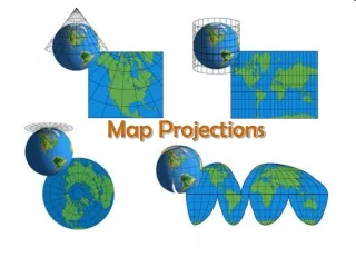
Classes of projections • Cylindrical • Planar (azimuthal) • Conical CS 128/ES 228 - Lecture 3a
Cylindrical projections • Meridians & parallels intersect at 90o • Often conformal • Least distortion along line of contact (typically equator) • Ex. Mercator- the ‘standard’ school map http://ioc.unesco.org/oceanteacher/resourcekit/Module2/GIS/Module/Module_c/module_c4.html CS 128/ES 228 - Lecture 3a
Transverse Mercator projection • Mercator is hopelessly poor away from the equator • Fix: rotate the projection 90° so that the line of contact is a central meridian (N-S) • Ex. Universal Transverse Mercator CS 128/ES 228 - Lecture 3a
Planar projections • a.k.a Azimuthal • Best for polar regions CS 128/ES 228 - Lecture 3a
Conical projections • Most accurate along “standard parallel” • Meridians radiate out from vertex (often a pole) • Ex. Albers Equal Area • Poor in polar regions – just omit those areas CS 128/ES 228 - Lecture 3a
Compromise projections • Robinson world projection • Based on a set ofcoordinates rather than a mathematical formula • Shape, area, and distance ok near origin and along equator • Neither conformal nor equivalent (equal area). Useful only for world maps http://ioc.unesco.org/oceanteacher/resourcekit/Module2/GIS/Module/Module_c/module_c4.html CS 128/ES 228 - Lecture 3a
More compromise projections CS 128/ES 228 - Lecture 3a
What if you’re interested in oceans? http://www.cnr.colostate.edu/class_info/nr502/lg1/map_projections/distortions.html CS 128/ES 228 - Lecture 3a
“But wait: there’s more …” http://www.dfanning.com/tips/map_image24.html All but upper left: http://www.geography.hunter.cuny.edu/mp/amuse.html CS 128/ES 228 - Lecture 3a
Buckminster Fuller’s “Dymaxion” CS 128/ES 228 - Lecture 3a