
Filtering
E N D
Presentation Transcript
Filtering EECS 442 – David Fouhey Fall 2019, University of Michigan http://web.eecs.umich.edu/~fouhey/teaching/EECS442_F19/ Note: I need some volunteers for a cheesy demonstration, please sit near the front if you’re willing.
Let’s Fix Things • We have noise in our image • Let’s replace each pixel with a weighted average of its neighborhood • Weights are filter kernel 1/9 1/9 1/9 Out 1/9 1/9 1/9 1/9 1/9 1/9 Slide Credit: D. Lowe
1D Case Signal/ Front Row 12 11 10 11 9 12 10 Filter/ David 1/3 1/3 1/3 11 10.66 10 10.66 10.33 Output
Applying a Linear Filter Input Filter Output I15 I16 I12 I13 I14 I11 O12 O13 O14 O11 I25 I26 I22 I23 I24 I21 I35 I36 I32 I33 I34 I31 O22 O23 O24 O21 F12 F13 F11 O32 O33 O34 O31 I45 I46 I42 I43 I44 I41 I55 I56 I52 I53 I54 I51 F22 F23 F21 F32 F33 F31
Applying a Linear Filter Input & Filter Output I15 I16 I12 I13 I14 I11 O11 I25 I26 I22 I23 I24 I21 I35 I36 I32 I33 I34 I31 F12 F13 F11 I45 I46 I42 I43 I44 I41 I55 I56 I52 I53 I54 I51 F22 F23 F21 F32 F33 F31 O11 = I11*F11 + I12*F12 + … + I33*F33
Applying a Linear Filter Input & Filter Output I15 I16 I12 I13 I14 I11 O11 O12 I25 I26 I22 I23 I24 I21 I35 I36 I32 I33 I34 I31 F12 F13 F11 I45 I46 I42 I43 I44 I41 I55 I56 I52 I53 I54 I51 F22 F23 F21 F32 F33 F31 O12 = I12*F11 + I13*F12 + … + I34*F33
Applying a Linear Filter Input Filter Output I15 I16 I12 I13 I14 I11 I25 I26 I22 I23 I24 I21 I35 I36 I32 I33 I34 I31 F12 F13 F11 I45 I46 I42 I43 I44 I41 I55 I56 I52 I53 I54 I51 F22 F23 F21 F32 F33 F31 How many times can we apply a 3x3 filter to a 5x6 image?
Applying a Linear Filter Input Filter Output I15 I16 I12 I13 I14 I11 O12 O13 O14 O11 I25 I26 I22 I23 I24 I21 I35 I36 I32 I33 I34 I31 O22 O23 O24 O21 F12 F13 F11 O32 O33 O34 O31 I45 I46 I42 I43 I44 I41 I55 I56 I52 I53 I54 I51 F22 F23 F21 F32 F33 F31 Oij = Iij*F11 + Ii(j+1)*F12 + … + I(i+2)(j+2)*F33
Painful Details – Edge Cases Convolution doesn’t keep the whole image. Suppose f is the image and g the filter. Full – any part of g touches f. Same – same size as f; Valid – only when filter doesn’t fall off edge. full same valid g g g g f f f g g g g g g g g f/g Diagram Credit: D. Lowe
Painful Details – Edge Cases What to about the “?” region? g ? ? ? ? g Symm: fold sides over f Circular/Wrap: wrap around pad/fill: add value, often 0 g g f/g Diagram Credit: D. Lowe
Painful Details – Does it Matter? (I’ve applied the filter per-color channel) Which padding did I use and why? Box Filtered ??? Input Image Box Filtered ??? Note – this is a zoom of the filtered, not a filter of the zoomed
Painful Details – Does it Matter? (I’ve applied the filter per-color channel) Box Filtered Zero Pad Input Image Box Filtered Symm Pad Note – this is a zoom of the filtered, not a filter of the zoomed
Practice with Linear Filters 0 0 0 ? 1 0 0 0 0 0 Original Slide Credit: D. Lowe
Practice with Linear Filters 0 0 0 1 0 0 0 0 0 Original The Same! Slide Credit: D. Lowe
Practice with Linear Filters 0 0 0 ? 0 1 0 0 0 0 Original Slide Credit: D. Lowe
Practice with Linear Filters 0 0 0 0 1 0 0 0 0 Original Shifted LEFT 1 pixel Slide Credit: D. Lowe
Practice with Linear Filters 1 0 0 ? 0 0 0 0 0 0 Original Slide Credit: D. Lowe
Practice with Linear Filters 1 0 0 0 0 0 0 0 0 Original Shifted DOWN 1 pixel Slide Credit: D. Lowe
Practice with Linear Filters 1/9 1/9 1/9 ? 1/9 1/9 1/9 1/9 1/9 1/9 Original Slide Credit: D. Lowe
Practice with Linear Filters 1/9 1/9 1/9 1/9 1/9 1/9 1/9 1/9 1/9 Original Blur (Box Filter) Slide Credit: D. Lowe
Practice with Linear Filters 1/9 0 1/9 0 1/9 0 ? 2 1/9 1/9 0 1/9 0 - 0 1/9 0 1/9 1/9 0 Original Slide Credit: D. Lowe
Practice with Linear Filters 0 1/9 0 1/9 1/9 0 2 1/9 0 1/9 1/9 0 - 1/9 0 0 1/9 0 1/9 Original Sharpened (Acccentuates difference from local average) Slide Credit: D. Lowe
Sharpening Slide Credit: D. Lowe
Properties – Linear Assume: I image f1, f2 filters Linear: apply(I,f1+f2) = apply(I,f1) + apply(I,f2) I is a white box on black, and f1, f2 are rectangles A( , + ) =A( , ) = A( , )+A( , ) = + = Note: I am showing filters un-normalized and blown up. They’re a smaller box filter (i.e., each entry is 1/(size^2))
Properties – Shift-Invariant Assume: I image, f filter Shift-invariant: shift(apply(I,f)) = apply(shift(I,f)) Intuitively: only depends on filter neighborhood A( , ) = A( , ) =
Painful Details – Signal Processing Often called “convolution”. Actually cross-correlation. Cross-Correlation (Original Orientation) Convolution (Flipped in x and y)
Properties of Convolution • Any shift-invariant, linear operation is a convolution (⁎) • Commutative: f ⁎ g = g ⁎ f • Associative: (f ⁎ g) ⁎ h = f ⁎ (g ⁎ h) • Distributes over +: f ⁎ (g + h) = f ⁎ g + f ⁎ h • Scalars factor out: kf⁎ g = f ⁎ kg = k (f ⁎ g) • Identity (a single one with all zeros): * = Property List: K. Grauman
Questions? • Nearly everything onwards is a convolution. • This is important to get right.
Smoothing With A Box Intuition: if filter touches it, it gets a contribution. Input Box Filter
Solution – Weighted Combination Intuition: weight contributions according to closeness to center. What’s this?
Recognize the Filter? It’s a Gaussian! 0.003 0.013 0.022 0.013 0.003 0.013 0.060 0.098 0.060 0.013 0.022 0.098 0.162 0.098 0.022 0.013 0.060 0.098 0.060 0.013 0.003 0.013 0.022 0.013 0.003
Smoothing With A Box & Gauss Still have some speckles, but it’s not a big box Input Box Filter Gauss. Filter
Gaussian Filters σ = 1 filter = 21x21 σ = 2 filter = 21x21 σ = 4 filter = 21x21 σ = 8 filter = 21x21 Note: filter visualizations are independently normalized throughout the slides so you can see them better
Applying Gaussian Filters Input Image (no filter)
Picking a Filter Size Too small filter → bad approximation Want size ≈ 6σ (99.7% of energy) Left far too small; right slightly too small! σ = 8, size = 21 σ = 8, size = 43
Runtime Complexity Image size = NxN = 6x6 Filter size = MxM = 3x3 I15 I16 for ImageY in range(N): for ImageX in range(N): for FilterY in range(M): for FilterX in range(M): … Time: O(N2M2) I12 I13 I14 I11 I25 I26 I22 I23 I24 I21 I35 I36 I32 I33 I34 I31 F12 F13 F11 I45 I46 I42 I43 I44 I41 I55 I56 I52 I53 I54 I51 F22 F23 F21 F32 F33 F31 I65 I66 I62 I63 I64 I61
Separability Conv(vector, transposed vector) → outer product Fx1 Fx2 Fx3 Fy1 Fx1 * Fy1 Fx2 * Fy1 Fx3 * Fy1 Fy2 Fx1 * Fy2 Fx2 * Fy2 Fx3 * Fy2 Fy3 Fx1 * Fy3 Fx2 * Fy3 Fx3 * Fy3 ⁎ =
Separability 1D Gaussian ⁎ 1D Gaussian = 2D Gaussian Image ⁎ 2D Gauss = Image ⁎ (1D Gauss ⁎ 1D Gauss ) = (Image ⁎ 1D Gauss) ⁎ 1D Gauss ⁎ =
Runtime Complexity Image size = NxN = 6x6 Filter size = Mx1 = 3x1 I15 I16 for ImageY in range(N): for ImageX in range(N): for FilterY in range(M): … for ImageY in range(N): for ImageX in range(N): for FilterX in range(M): … Time: O(N2M) I12 I13 I14 I11 F1 I25 I26 I22 I23 I24 I21 F2 I35 I36 I32 I33 I34 I31 F3 I45 I46 I42 I43 I44 I41 I55 I56 I52 I53 I54 I51 I65 I66 I62 I63 I64 I61 What are my compute savings for a 13x13 filter?
Why Gaussian? Gaussian filtering removes parts of the signal above a certain frequency. Often noise is high frequency and signal is low frequency.
Why Does This Fail? Means can be arbitrarily distorted by outliers Signal 10 12 11 1000 8 9 12 10 0.1 0.8 0.1 Filter 109.8 10.3 801.9 107.3 9.2 11.5 Output What else is an “average” other than a mean?