Python & Web Mining
Learn how to classify and filter documents based on their content using Python and web mining techniques. Explore the classification of binary and n-ary documents, spam elimination methods, feature extraction, and classifier training. Enhance your skills with examples and solutions.

Python & Web Mining
E N D
Presentation Transcript
Python & Web Mining Lecture 5 10-03-12 Old Dominion University Department of Computer Science CS 495 Fall 2012 Presented & Prepared by: Justin F. Brunelle jbrunelle@cs.odu.edu Hany SalahEldeen Khalil hany@cs.odu.edu Hany SalahEldeen CS495 – Python & Web Mining Fall 2012
Chapter 6: “Document Filtering” Hany SalahEldeen CS495 – Python & Web Mining Fall 2012
In a nutshell: It is classifying documents based on their content. This classification could be binary (good/bad, spam/not-spam) or n-ary (school-related-emails, work-related, commercials…etc) Document Filtering Hany SalahEldeen CS495 – Python & Web Mining Fall 2012
Eliminate spam. • Removing unrelated comments in forums and public message boards. • Classifying social /work-related emails automatically. • Forwarding information-request emails to the expert who is most capable of answering the email. Why do we need Document filtering? Hany SalahEldeen CS495 – Python & Web Mining Fall 2012
First it was rule-based classifiers: • Overuse capital letters • Words related to pharmaceutical products • Garish HTML colors Spam Filtering Hany SalahEldeen CS495 – Python & Web Mining Fall 2012
Easy to trick by just avoiding patterns of capital letters…etc. • What is considered spam varies from one to another. • Ex: Inbox of a medical rep Vs. email of a house-wife. Cons of using Rule-based classifiers Hany SalahEldeen CS495 – Python & Web Mining Fall 2012
Develop programs that learn. • Teach them the differences and how to recognize each class by providing examples of each class. Solution Hany SalahEldeen CS495 – Python & Web Mining Fall 2012
We need to extract features from documents to classify them. • Feature: Is anything that you can determine as being either present or absent in the item. Features Hany SalahEldeen CS495 – Python & Web Mining Fall 2012
item = document • feature = word • classification = {good|bad} Definitions Hany SalahEldeen CS495 – Python & Web Mining Fall 2012
Dictionary Building Hany SalahEldeen CS495 – Python & Web Mining Fall 2012
Remember: • Removing capital letters reduce the total number of features by removing the SHOUTING style. • Size of the features also is crucial (using entire email as feature Vs. each letter a feature) Dictionary Building Hany SalahEldeen CS495 – Python & Web Mining Fall 2012
It is designed to start off very uncertain. • Increase certainty upon learning features. Classifier Training Hany SalahEldeen CS495 – Python & Web Mining Fall 2012
Classifier Training Hany SalahEldeen CS495 – Python & Web Mining Fall 2012
It’s a number between 0-1 indicating how likely an event is. Probabilities Hany SalahEldeen CS495 – Python & Web Mining Fall 2012
‘quick’ appeared in 2 documents as good and the total number of good documents is 3 Probabilities Hany SalahEldeen CS495 – Python & Web Mining Fall 2012
Pr(A|B) = “probability of A given B” fprob(quick|good) = “probability of quick given good” = (quick classified as good) / (total good items) = 2 / 3 Conditional Probabilities Hany SalahEldeen CS495 – Python & Web Mining Fall 2012
Using the info we seen so far makes it extremely sensitive in early training stages • Ex: “money” • Money appeared in casino training document as bad • It appears with probability = 0 for good which is not right! Starting with Reasonable guess Hany SalahEldeen CS495 – Python & Web Mining Fall 2012
Start for instance with 0.5 probability for each feature • Also decide the weight chosen for the assumed probability you will take. Solution: Start with assumed probability Hany SalahEldeen CS495 – Python & Web Mining Fall 2012
define an assumed probability of 0.5 then weightedprob() returns the weighted mean of fprob and the assumed probability weightedprob(money,good) = (weight * assumed + count * fprob()) / (count + weight) = (1*0.5 + 1*0) / (1+1) = 0.5 / 2 = 0.25 (double the training) = (1*0.5 + 2*0) / (2+1) = 0.5 / 3 = 0.166 >>> cl.weightedprob('money','good',cl.fprob) 0.25 >>> docclass.sampletrain(cl) Nobody owns the water. the quick rabbit jumps fences buy pharmaceuticals now make quick money at the online casino the quick brown fox jumps >>> cl.weightedprob('money','good',cl.fprob) 0.16666666666666666 >>> cl.fcount('money','bad') 3.0 >>> cl.weightedprob('money','bad',cl.fprob) 0.5 Pr(money|bad) remains = (0.5 + 3*0.5) / (3+1) = 0.5 >>> cl.fprob('money','bad') 0.5 >>> cl.fprob('money','good') 0.0 we have data for bad, but should we start with 0 probability for money given good? Assumed Probability Hany SalahEldeen CS495 – Python & Web Mining Fall 2012
Move from terms to documents: Pr(document) = Pr(term1) * Pr(term2) * … * Pr(termn) Naïvebecause we assume all terms occur independently we know this is as simplifying assumption; it is naïve to think all terms have equal probability for completing this phrase: “Shave and a hair cut ___ ____” Bayesianbecause we use Bayes’ Theorem to invert the conditional probabilities Naïve Bayesian Classifier Hany SalahEldeen CS495 – Python & Web Mining Fall 2012
Given our training data, we know: Pr(feature|classification) What we really want to know is: Pr(classification|feature) Bayes’ Theorem* : Pr(A|B) = Pr(B|A) Pr(A) / Pr(B) Pr(good|doc) = Pr(doc|good) Pr(good) / Pr(doc) * http://en.wikipedia.org/wiki/Bayes%27_theorem Bayes Theorem we skip this since it is the same for each classification Or: we know how to calculate this #good / #total Hany SalahEldeen CS495 – Python & Web Mining Fall 2012
>>> import docclass >>> cl=docclass.naivebayes(docclass.getwords) >>> docclass.sampletrain(cl) Nobody owns the water. the quick rabbit jumps fences buy pharmaceuticals now make quick money at the online casino the quick brown fox jumps >>> cl.prob('quick rabbit','good') quick rabbit 0.15624999999999997 >>> cl.prob('quick rabbit','bad') quick rabbit 0.050000000000000003 >>> cl.prob('quick rabbit jumps','good') quick rabbit jumps 0.095486111111111091 >>> cl.prob('quick rabbit jumps','bad') quick rabbit jumps 0.0083333333333333332 Our Bayesian Classifier we use these values only for comparison, not as “real” probabilities Hany SalahEldeen CS495 – Python & Web Mining Fall 2012
http://en.wikipedia.org/wiki/Naive_Bayes_classifier#Testing Bayesian Classifier Hany SalahEldeen CS495 – Python & Web Mining Fall 2012
>>> cl.prob('quick rabbit','good') quick rabbit 0.15624999999999997 >>> cl.prob('quick rabbit','bad') quick rabbit 0.050000000000000003 >>> cl.classify('quick rabbit',default='unknown') quick rabbit u'good' >>> cl.prob('quick money','good') quick money 0.09375 >>> cl.prob('quick money','bad') quick money 0.10000000000000001 >>> cl.classify('quick money',default='unknown') quick money u'bad' >>> cl.setthreshold('bad',3.0) >>> cl.classify('quick money',default='unknown') quick money 'unknown' >>> cl.classify('quick rabbit',default='unknown') quick rabbit u'good' Classification Thresholds only classify something as bad if it is 3X more likely to be bad than good Hany SalahEldeen CS495 – Python & Web Mining Fall 2012
>>> for i in range(10): docclass.sampletrain(cl) >>> cl.prob('quick money','good') quick money 0.016544117647058824 >>> cl.prob('quick money','bad') quick money 0.10000000000000001 >>> cl.classify('quick money',default='unknown') quick money u'bad' >>> cl.prob('quick rabbit','good') quick rabbit 0.13786764705882351 >>> cl.prob('quick rabbit','bad') quick rabbit 0.0083333333333333332 >>> cl.classify('quick rabbit',default='unknown') quick rabbit u'good' Classification Thresholds…cont Hany SalahEldeen CS495 – Python & Web Mining Fall 2012
Normalize the frequencies for each category e.g., we might have far more “bad” training data than good, so the net cast by the bad data will be “wider” than we’d like Calculate normalized Bayesian probability, then fit the result to an inverse chi-square function to see what is the probability that a random document of that classification would have those features (i.e., terms) Fisher Method Hany SalahEldeen CS495 – Python & Web Mining Fall 2012
>>> import docclass >>> cl=docclass.fisherclassifier(docclass.getwords) >>> cl.setdb('mln.db') >>> docclass.sampletrain(cl) >>> cl.cprob('quick','good') 0.57142857142857151 >>> cl.fisherprob('quick','good') quick 0.5535714285714286 >>> cl.fisherprob('quick rabbit','good') quick rabbit 0.78013986588957995 >>> cl.cprob('rabbit','good') 1.0 >>> cl.fisherprob('rabbit','good') rabbit 0.75 >>> cl.cprob('quick','good') 0.57142857142857151 >>> cl.cprob('quick','bad') 0.4285714285714286 Fisher Example Hany SalahEldeen CS495 – Python & Web Mining Fall 2012
>>> cl.cprob('money','good') 0 >>> cl.cprob('money','bad') 1.0 >>> cl.cprob('buy','bad') 1.0 >>> cl.cprob('buy','good') 0 >>> cl.fisherprob('money buy','good') money buy 0.23578679513998632 >>> cl.fisherprob('money buy','bad') money buy 0.8861423315082535 >>> cl.fisherprob('money quick','good') money quick 0.41208671548422637 >>> cl.fisherprob('money quick','bad') money quick 0.70116895256207468 Fisher Example Hany SalahEldeen CS495 – Python & Web Mining Fall 2012
>>> cl.fisherprob('quick rabbit','good') quick rabbit 0.78013986588957995 >>> cl.classify('quick rabbit') quick rabbit u'good' >>> cl.fisherprob('quick money','good') quick money 0.41208671548422637 >>> cl.classify('quick money') quick money u'bad' >>> cl.setminimum('bad',0.8) >>> cl.classify('quick money') quick money u'good' >>> cl.setminimum('good',0.4) >>> cl.classify('quick money') quick money u'good' >>> cl.setminimum('good',0.42) >>> cl.classify('quick money') quick money Classification with Inverse Chi-Square in practice, we’ll tolerate false positives for “good” more than false negatives for “good” -- we’d rather see a mesg that is spam rather than lose a mesg that is not spam. this version of the classifier does not print “unknown” as a classification Hany SalahEldeen CS495 – Python & Web Mining Fall 2012
Reduces the signal – to – noise ratios Assumes document occur with normal distribution Estimates differences in corpus size with X-squared “Chi”-squared is a “goodness-of-fit” b/t an observed distribution and theoretical distribution Utilizes confidence interval & std. dev. estimations for a corpus http://en.wikipedia.org/w/index.php?title=File:Chi-square_pdf.svg&page=1 Fisher -- Simplified Hany SalahEldeen CS495 – Python & Web Mining Fall 2012
Pick one question from the end of the chapter. • Implement the function and state briefly the differences. • Utilize the python files associated with the class if needed. • Deadline: Next week Assignment 4 Hany SalahEldeen CS495 – Python & Web Mining Fall 2012

