Download
1 / 127
1.84k likes | 3.23k Vues
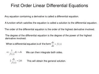
Chapter 2 Theory of First Order Differential Equations. Shurong Sun University of Jinan Semester 1, 2011-2012. 1 Existence-uniqueness theorem ( Picard’s Method of Successive Approximations ). Consider the initial-value problem. (1).

E N D
Chapter 2Theory of First Order Differential Equations Shurong Sun University of Jinan Semester 1, 2011-2012
1Existence-uniqueness theorem (Picard’s Method of Successive Approximations) Consider the initial-value problem (1) Q1. How to know that the IVP (1) actually has a solution if we can’t exhibit it? Q2. How do we know that there is only one solution y(t) of (1)?
The short answer to the question, how do youknow the equation has a solution, is ‘Picarditeration’. Picard’s Existence and Uniqueness Theorem is one of the most important theorems in ODE! Why is Picard’s Theorem so important? Iteration means to do something over and over.
(i) Rewrite the differential equation as an integral equation: (ii) Pick a function satisfying the initial condition. Pick Define Then we iterate: define
define and having defined This gives a sequence of functions Picard iteration The solution is when Picard iteration works. Intuitively, is the solution since
and But then
Remark: Was that a foolproof proof? Almost, but the formula is called ‘taking the limit under the integral sign’ and it is not always correct. We need to add some further conditions on f to make it work. But basically this is the idea.
Theorem 1.1 (Existence and uniqueness for the Cauchy problem) Let and suppose that • is continuous, • satisfies a Lipschitz condition with respect to y. Then the Cauchy problem (1) has a unique solution on where
Proof of the Theorem We will prove the theorem in five steps: • Show that the initial value problem (1) is equivalent to the integral equation (2)
(ii) Set up a sequence of Picard iteration and show that they are well defined. (iii) Show that our sequence of Picard iteration converges uniformly. (iv) Show that the function to which our sequence converges is a solution to the IVP. (v) Show that this solution is unique.
(i) The initial-value problem (1) is equivalent to the integral equation (2) Specifically, if y(t) satisfies (1), then (2) Hence
Conversely, if y(t) is continuous and satisfies (2), then Moreover, Therefore, y(t) is a solution of (1) if, and only if, it is a continuous solution of (2).
(ii)Construction of the approximating sequence Let us start by guessing a solution of (2). The simplest possible guess is To check whether is a solution, we compute If then is indeed a solution of (2). If not, then we try as our next guess.
To check whether is a solution, we compute and so on. In this manner, we define a sequence of functions (3) where are called successive approximation, These functions or Picard iteration, after the French mathematician Picard who first discovered them.
Define the sequence of Picard iteration as To ensure that Picard iteration are well defined it is sufficient to ensure that each stays within [-b,b], that is (4) It’s convenient to assume a similar proof will hold for
We prove (4) by induction on n. Observe first that (4) is obviously true for n=0, since Next, we must show that (4) is true for n=j+1 if it is true for n=j. But this follows immediately, for then . for
(iii) We now show that our sequence of Picard iteration converges uniformly for t in the interval This is accomplished by writing in the form Clearly, the sequence converges if, and only if, the infinite series converges .
To prove the infinite series converges, it suffices to show that Observe that (5)
Setting n=1 in (5) gives This, in turn, implies that
Proceeding inductively, we see that Therefore, for Consequently, converges uniformly on the interval since
We denote the limit of the sequence by y(t), which is continuous on (iv) Prove that y(t) satisfies the initial-value problem (1) We will show that y(t) satisfies the integral equation To this end, recall that the Picard iteration are defined recursively through the equation (6) Taking limits of both sides of (6) gives
Note that converges uniformly to f(s,y(s)) on since and converges uniformly to y(t) on Then one can exchange integral and the limit. Thus and y(t) satisfies
(v) Show that the solution is unique. (i) Let z(t) be also a solution of (2). By induction we show that (7) We have and therefore which (7) holds for n = 0.
If (7) holds for n − 1 we have and this proves for all
Consequently, since This implies that converges uniformly to z(t) on And so
(v) (ii) It remains to prove uniqueness of the solution. Let y(t) and z(t) be two solutions of (2). By recurrence we show that (7) We have and therefore which (7) for k = 0.
If (7) for k − 1 holds we have and this proves for all
Consequently, since This implies that
Remark: (1) Geometrically, this means the graph of is constrained to lie in the shaded region shown below.
Remark: (2) Geometrically, this means the graph of is constrained to lie in the shaded region shown below.
(3) If is continuous in the rectangle A , then f satisfies a Lipschitz condition, since where Note that f satisfies a Lipschitz condition is continuous. For example: f(t,y)=|y|.
Corollary : Let f and be continuous in the rectangle Compute Then the initial problem has a unique solution y(t) on the interval
Example 1.1 Show that the solution y(t) of the initial-value problem exists for and in this interval, Solution: Let Computing we see that y(t) exists for and in this interval,
Remark (4)The initial value problem (IVP) where has a unique solution valid on [a, b].
Proof (Method I) The unique solution is to the IVP is
Method II Successive approximation • Show that the initial value problem (1) is equivalent to the integral equation (2) Specifically, y(t) is a solution of (1) on [a,b] if, and only if, it is a continuous solution of (2) on [a,b].
(ii)Construction of the approximating sequence Then are well defined on [a,b] for all (iii) Show that the sequence of Picard iteration converges uniformly on the interval converges if, and only if, the infinite series converges .
Take Then (iv) Show that the limit of the sequence is a continuous solution to the integral equation (2) on [a,b]. (v) Show that this solution is unique. Take Then
Theorem 1.2 (Peano 1890) Let and suppose that is continuous with Set Then the Cauchy problem (1) has a solution on
Estimates of error and approximate calculation The method of Picard iteration not only give the solution but also found functions which approximate it well, i.e. Let y(t) be the exact solution of the IVP and the Picard scheme for solving this is
If we make in approximating the solution y(t) by then the error is called the nth approximate solution to the IVP.
Example1.2 Let (i) Determine the interval of existence that the Existence Theorem predicts for the solution y(x) of the initial-value problem (ii) Determine an approximate solution of the IVP above such that the error is less than 0.05.
Solution: the existence and uniqueness theorem holds. From the Existence Theorem, has a unique solution on [-h,h]. Here Thus, the interval of solution is
Since we can take Take then .
The successive approximates are: is the approximate solution desired,
Example 1.3The initial value problem is equivalent to solving the integral equation Let We obtain