Download
1 / 56
600 likes | 998 Vues
Explore methods for linear DE: Homogeneous, Nonhomogeneous, Boundary Value Problems, and Solution Techniques using laplace transform, series methods, and more.

E N D
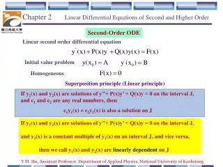
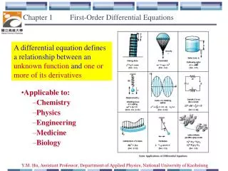
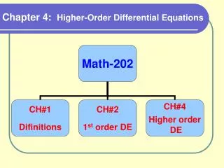
Chapter 4 Higher Order Differential Equations Highest differentiation: , n > 1 Most of the methods in Chapter 4 are applied for the linear DE.
附錄四DE 的分類 Homogeneous Constant coefficients Nonhomogeneous Linear Homogeneous Cauchy-Euler DE Nonhomogeneous Homogeneous Others Nonhomogeneous Nonlinear
附錄五 Higher Order DE 解法 reduction of order homogeneouspart auxiliary function linear Cauchy-Euler “guess” method particular solution annihilator variation of parameters multiple linear DEs elimination method reduction of order nonlinear Taylor series numerical method Laplace transform series solution both (but mainly linear) Fourier series transform Fourier cosine series Fourier sine series Fourier transform
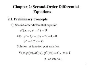
4-1 Linear Differential Equations: Basic Theory 4.1.1 Initial-Value and Boundary Value Problems 4.1.1.1 The nth Order Initial Value Problem i.e., the nth order linear DE with the constraints at the same point ………….. ……………….. n initial conditions
Theorem 4.1.1 For an interval I that contains the point x0 If a0(x), a1(x), a2(x), ……., an−1(x ), an(x) are continuous at x = x0 an(x0) 0 (很像Section 2-3 當中沒有 singular point 的條件) then for the problem on page 139, the solution y(x) exists and is uniqueon the interval I that contains the point x0 (Interval I的範圍,取決於何時 an(x) = 0以及 何時 ak(x) (k = 0 ~ n) 不為continuous) Otherwise, the solution is either non-unique or does not exist. (infinite number of solutions) (no solution)
Example 1 (text page 119) Example 2 (text page 120) 有無限多組解 c為任意之常數
比較: There is only one solution x (0, ) Note: The initial value can also be the form as: (general initial condition)
4.1.1.2 nth Order Boundary Value Problem Boundary conditions are specified at different points 比較:Initial conditions are specified at the same points 例子: subject to 或 或 An nth order linear DE with n boundary conditions may have a unique solution, no solution, or infinite number of solutions.
Example 3 (text page 120) solution: (1) c2 is any constant (infinite number of solutions) (2) (unique solution)
4.1.2 Homogeneous Equations 4.1.2.1 Definition g(x) = 0 homogeneous g(x) 0 nonhomogeneous 重要名詞:Associated homogeneous equation The associated homogeneous equation of a nonhomogeneous DE: Setting g(x) = 0 • Review: Section 2-3, pages 53, 55
4.1.2.2 New Notations Notation: 可改寫成 可改寫成 可再改寫成
4.1.2.3 Solution of the Homogeneous Equation [Theorem 4.1.5] For an nth order homogeneous linear DE L(y) = 0, if y1(t), y2(t), ….., yn(t) are the solutions of L(y) = 0 y1(t), y2(t), ….., yn(t) are linearly independent then any solution of the homogeneous linear DE can be expressed as: 可以和矩陣的概念相比較
From Theorem 4.1.5: An nth orderhomogeneouslinearDE has n linearly independent solutions. Find n linearly independent solutions == Find all the solutions of an nth order homogeneous linear DE y1(t), y2(t), ….., yn(t): fundamental set of solutions : general solution of the homogenous linear DE (又稱做 complementary function) 也是重要名詞
Definition 4.1 Linear Dependence / Independence If there is no solution other than c1 = c2 = ……. = cn = 0 for the following equality then y1(t), y2(t), ….., yn(t) are said to be linearly independent. Otherwise, they are linearly dependent. 判斷是否為 linearly independent 的方法: Wronskian
Definition 4.2 Wronskian linearly independent
4.1.2.4 Examples Example 9 (text page 127) y1 = ex, y2 = e2x, and y3 = e3x are three of the solutions Since Therefore, y1, y2, and y3 are linear independent for any x general solution: x (−, )
4.1.3 Nonhomogeneous Equations (可和 page 55 相比較) Nonhomogeneous linear DE Part 1 Part 2 Associated homogeneous DE particular solution (any solution of the nonhomogeneous linear DE) findn linearly independent solutions general solution of the nonhomogeneous linear DE
Theorem 4.1.6 general solution of a nonhomogeneous linear DE general solution of the associated homogeneous function (complementary function) particular solution (any solution) of the nonhomogeneous linear DE general solution of the nonhomogeneous linear DE
Example 10 (text page 128) Particular solution Three linearly independent solution , , Check by Wronskian (Example 9) General solution:
Theorem 4.1.7 Superposition Principle If is the particular solution of is the particular solution of : is the particular solution of then is the particular solution of
Example 11 (text page 129) is a particular solution of is a particular solution of is a particular solution of is a particular solution of
4.1.4 名詞 • initial conditions, boundary conditions (pages 139, 143) (重要名詞) • associated homogeneous equation , complementary function (page 145)(重要名詞) • fundamental set of solutions (page 148) • Wronskian (page 150) • particular solution (page 152) • general solution of the homogenous linear DE (page 148) • general solution of the nonhomogenous linear DE (page 152)
4.1.5 本節要注意的地方 (1) Most of the theories in Section 4.1 are applied to the linearDE (2) 注意 initial conditions和 boundary conditions之間的不同 (3) 快速判斷 linear independent
(補充 1) Theorem 4.1.1 的解釋 ……………….. When an(x0) 0 find y(n)(x0) find y(n−1)(x0+) (根據 , )
以此類推 find y(n−2)(x0+) find y(n−3)(x0+) : : find y(x0+) find y(n)(x0+) find y(n−1)(x0+2) find y(n−2)(x0+2)
: : find y(x0+2) 以此類推,可將 y(x0+3), y(x0+4), y(x0+5), …………… 以至於將 y(x) 所有的值都找出來。 (求 y(x) for x > x0時, 用正的 值, 求 y(x) for x < x0時, 用負的 值)
Requirement 1: a0(x), a1(x), a2(x), ……., an−1(x ), an(x) are continuous 是為了讓 ak(x0+m) 皆可以定義 Requirement 2: an(x) 0是為了讓 ak(x0+m) /an(x0+m) 不為無限大
4-2 Reduction of Order 4.2.1 適用情形 (1) (2) (3) Suitable for the 2nd orderlinearhomogeneous DE (4) One of the nontrivial solution y1(x) has been known.
4.2.2 解法 假設 先將DE 變成 Standard form If y(x) = u(x) y1(x) , (比較 Section 2-3) zero
set w = u' multiplied by dx/(y1w) separable variable(with 3 variables)
We can set c1 = 1 and c2 = 0 (因為我們算 u(x) 的目的,只是為了要算出與 y1(x) 互相independent 的另一個解)
4.2.3 例子 Example 1 (text page 132) We have known that y1 = ex is one of the solution P(x) = 0 Specially, set c = –2, (y2(x) 只要 independent of y1(x) 即可 所以 c的值可以任意設) General solution:
Example 2 (text page 133) (將課本 x的範圍做更改) when x (−, 0) We have known that y1 = x2 is one of the solution Note: the interval of x If x (0, ) (x > 0), 如課本 If x < 0,
4.2.4 本節需注意的地方 (1) 記住公式 (2) 若不背公式 (不建議),在計算過程中別忘了對 w(x) 做積分 (3) 別忘了 P(x) 是 “standard form” 一次微分項的 coefficient term (4) 同樣有 singular point 的問題 (5) 因為 y2(x) 是 homogeneous linear DE 的 “任意解”,所以計算時,常數的選擇以方便為原則 (6) 由於 的計算較複雜且花時間,所以要多加練習 多算習題
附錄七 Linear DE 解法的步驟 (參照講義 page 152) Step 1: Find the general solution (i.e., the complementary function ) of the associated homogeneous DE (Sections 4-2, 4-3, 4-7) Step 2: Find the particular solution (Sections 4-4, 4-5, 4-6) Step 3: Combine the complementary function and the particular solution Extra Step: Consider the initial (or boundary) conditions
4-3 Homogeneous Linear Equations with Constant Coefficients 本節使用 auxiliary equation的方法來解 homogeneous DE KK: [ ] 4-3-1 限制條件 限制條件: (1) homogeneous (2) linear (3) constant coefficients a0, a1, a2, …. , an are constants (the simplest case of the higher order DEs)
4-3-2 解法 解法核心: Suppose that the solutions has the form ofemx Example: y''(x) 3y'(x) + 2y(x) = 0 Set y(x) = emx, m2 emx 3m emx + 2 emx = 0 m2 3m + 2 = 0 solve m 可以直接把 n次微分用 mn取代,變成一個多項式 這個多項式被稱為 auxiliary equation
解法流程 Step 1-1 auxiliary function Step 1-1 Find n roots , m1, m2, m3, …., mn (If m1, m2, m3, …., mnare distinct) Step 1-2 n linearly independent solutions (有三個 Cases) Step 1-3 Complementaryfunction
4-3-3 Three Cases for Roots (2nd Order DE) roots solutions Case 1m1 m2, m1, m2 are real (其實 m1, m2不必限制為 real)
Case 2m1= m2 (m1 and m2 are of course real) First solution: Second solution: using the method of “Reduction of Order”
Case 3m1 m2 , m1 and m2 are conjugate and complex Solution: Another form: set c1 = C1 + C2 and c2 = jC1−jC2 c1 and c2 are some constant
Example 1 (text page 137) (a) 2m2− 5m− 3 = 0, m1 = −1/2, m2 = 3 (b) m2 − 10m + 25 = 0, m1 = 5, m2 = 5 (c) m2 + 4m + 7 = 0,
4-3-4 Three + 1 Cases for Roots (Higher Order DE) For higher order case auxiliary function: roots:m1, m2, m3, …., mn (1) If mpmq for p = 1, 2, …, n and p q (也就是這個多項式在 mq的地方只有一個根) then is a solution of the DE. (2)If the multiplicities of mq is k (當這個多項式在 mq的地方有 k個根), are the solutions of the DE. 重覆次數
(3) If both + j and −j are the roots of the auxiliary function, then are the solutions of the DE. (4) If the multiplicities of + j is k and the multiplicities of − j is also k,then are the solutions of the DE.
Note: If + j is a root of a real coefficient polynomial, then −j is also a root of the polynomial. a0, a1, a2, …. , an are real
Example 3 (text page 138) Solve Step 1-1 m1 = 1, m2 = m3 = 2 Step 1-2 3 independent solutions: Step 1-3 general solution: