Understanding Higher-Order Differential Equations Theory
990 likes | 1.59k Vues
Learn about linear equations, homogeneous equations, undetermined coefficients, variation of parameters, and linear models. Understand important concepts such as existence and uniqueness of solutions, linear operators, superposition principles, and Wronskian. Explore linear dependence, linear independence, and fundamental sets of solutions with examples.

Understanding Higher-Order Differential Equations Theory
E N D
Presentation Transcript
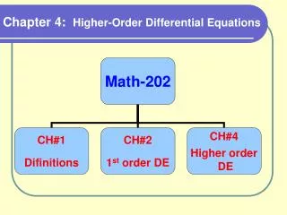
CHAPTER 3 Higher-Order Differential Equations
Contents • 3.1 Preliminary Theory: Linear Equations • 3.3 Homogeneous Linear Equations with Constant Coefficients • 3.4 Undetermined Coefficients • 3.5 Variation of Parameters • 3.8 Linear Models: Initial-Value Problems
3.1 Preliminary Theory: Linear Equ. • Initial-value ProblemAn initial value problem for nth-order linear DE iswith (1)as n initial conditions.
THEOREM 3.1 Existence and Uniqueness Let an(x), an-1(x), …, a0(x),and g(x)be continuous on I, an(x) 0for all x on I. If x = x0 is a point in this interval, then a solution y(x)of (1) exists on the interval and is unique.
Example 1 • The problem possesses the trivial solution y = 0. Since this DE with constant coefficients, from Theorem 3.1, hence y = 0 is the only one solution on any interval containing x = 1.
The following DE (6)is homogeneous; (7)with g(x)0, is nonhomogeneous.
Differential Operators • Let dy/dx = Dy. This symbol D is called a differential operator. We define an nth-order differential operator as (8)In addition, we have (9)so the differential operator L is a linear operator. • Differential EquationsWe can simply write the n-th order linear DEs as L(y) = 0andL(y) = g(x)
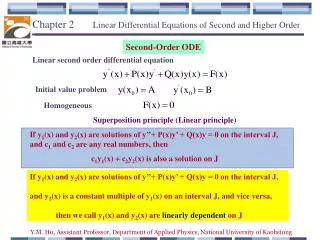
THEOREM 3.2 Let y1, y2, …, ynbe n solutions of the homogeneous nth-order differential equation (6) on an interval I. Then the linear combinationy = c1y1(x) + c2y2(x)+ …+ cnyn(x)where the ci, i = 1, 2, …, n are arbitrary constants, is also a solution on the interval. Superposition Principles – Homogeneous Equations
COROLLARY Corollaries to Theorem 3.2 (A) y = cy1 is also a solution if y1is a solution. (B) A homogeneous linear DE always possesses the trivial solution y = 0.
DEFINITION 3.1 A set of f1(x), f2(x), …, fn(x)is linearly dependent on an interval I, if there exists constants c1, c2, …, cn, not all zero, such thatc1f1(x) + c2f2(x) + … + cn fn(x) = 0If not linearly dependent, it is linearly independent. Linear Dependence and Linear Independence Linear Dependence and Independence
In other words, if the set islinearly independent, then c1f1(x) + c2f2(x) + … + cn fn(x) = 0implies c1 = c2 = … = cn= 0 • Referring to Fig 3.3, neither function is a constant multiple of the other, then these two functions are linearly independent.
Example 5 • The functions f1 = cos2 x, f2 = sin2x, f3 = sec2x, f4 =tan2x are linearly dependent on the interval (-/2, /2) sincec1 cos2 x +c2 sin2x +c3 sec2x +c4 tan2x = 0when c1 = c2 = 1, c3 = -1, c4 = 1.
Example 6 • The functions f1 = x½+ 5,f2 = x½ + 5x, f3 = x – 1,f4 = x2 are linearly dependent on the interval (0, ), since f2 = 1 f1 + 5 f3 + 0 f4
DEFINITION 3.2 Suppose each of the functions f1(x), f2(x), …, fn(x) possesses at least n – 1 derivatives. The determinantis called the Wronskian of the functions. Wronskian
THEOREM 3.3 Let y1(x), y2(x), …, yn(x) be solutions of the nth-order homogeneous DE (6) on an interval I. This set of solutions is linearly independent if and on if W(y1, y2, …, yn) 0 for every x in the interval. Criterion for Linear Independence Corollary 3.3 IfW(y1, y2, …, yn) 0 for some x in the interval then y1, y2, …, yn are linearly independent in the interval. If W(y1, y2, …, yn) = 0 for some x in the interval then y1, y2, …, yn are linearly dependent in the interval. . . .
DEFINITION 3.3 Any set y1(x), y2(x), …, yn(x) of n linearly independent solutions is said to be a fundamental set of solutions. Fundamental Set of a Solution
THEOREM 3.4 There exists a fundamental set of solutions for (6) on an interval I. Existence of a Fundamental Set THEOREM 3.5 Let y1(x), y2(x), …, yn(x) be a fundamental set of solutions of homogeneous DE (6) on an interval I. Then the general solution isy = c1y1(x) + c2y2(x) + … + cnyn(x) where ci are arbitrary constants. General Solution – Homogeneous Equations
Example 7 • The functions y1 = e3x, y2 = e-3xare solutions of y” –9y = 0on (-, )Now for every x. So y = c1y1 + c2y2is the general solution.
Example 8 • The functions y = 4sinh 3x - 5e3x is a solution of example 7 (Verify it). Observe = 4 sinh 3x – 5e-3x
Example 9 • The functions y1= ex,y2 = e2x , y3 = e3xare solutions of y’’’ –6y” + 11y’ –6y = 0on (-, ). Sincefor everyrealvalue of x. So y = c1ex + c2e2x + c3e3xis the general solution on (-, ).
THEOREM 3.6 Any ypfree of parameters satisfying (7) is called a particular solution. If y1(x), y2(x), …, yn(x) be a fundamental set of solutions of (6), then the general solution of (7) isy= c1y1 + c2y2 +… +cnyn + yp (10) General Solution – Nonhomogeneous Equations • Complementary Function: yy = c1y1 + c2y2 +… +cnyn +yp = yc + yp = complementary + particular
Example 10 • The function yp= -(11/12) –½ xis a particular solution of (11)From previous discussions, the general solution of (11) is
THEOREM 3.7 Given (12)where i = 1, 2, …, k. If ypi denotes a particular solution corresponding to the DE (12) with gi(x), then (13)is a particular solution of (14)
Example 11 • We findyp1 = -4x2 is a particular solution ofyp2 = e2xis a particular solution ofyp3 = xexis a particular solution of From Theorem 3.7, is a solution of
Note: • If ypi is a particular solution of (12), then is also a particular solution of (12) when the right-hand member is
3.3 Homogeneous Linear Equation with Constant Coefficients • Introduction: (1)where ai are constants, an 0. • Auxiliary Equation (Characteristic Equation):For n = 2, (2)Try y = emx, then (3)is called an auxiliary equation or characteristic equation.
From (3) the two roots are(1) b2 – 4ac > 0: two distinct real numbers.(2) b2 – 4ac = 0: two equal real numbers.(3) b2 – 4ac < 0: two conjugate complex numbers.
Case 1: Distinct real rootsThe general solution is (why?) (4) • Case 2: Repeated real roots, (why?) (5)The general solution is (why?) (6)
Case 3: Conjugate complex rootsWe write , a general solution is From Euler’s formula: and(7) and
Since is a solution then setC1= C1 = 1and C1 = 1, C2 = -1 , we have two solutions: So, ex cos x and exsin x are a fundamental set of solutions, that is, the general solution is(8)
Example 1 • Solve the following DEs: (a) (b) (c)
Example 2 Solve Solution:See Fig 3.4.
Higher-Order Equations • Given (12)we have (13)as an auxiliary equation (or characteristic equation).
Example 3 Solve Solution:
Example 4 Solve Solution:
Repeated complex roots • If m1= + i is a complex root of multiplicity k, then m2= − i is also a complex root of multiplicity k. The 2k linearly independent solutions:
3.4 Undetermined Coefficients • IntroductionIf we want to solve the nonhomogeneous linear DE (1)we have to find y = yc + yp. Thus we introduce the method of undetermined coefficients to solve for yp.
Example 1 Solve Solution: We can get ycas described in Sec 3.3. Now, we want to find yp. Since the right side of the DE is a polynomial, we setAfter substitution, 2A + 8Ax + 4B – 2Ax2 – 2Bx – 2C = 2x2– 3x + 6
Example 1 (2) Then
Example 2 Find a particular solution of Solution: Let yp = A cos 3x + B sin 3xAfter substitution, Then
Example 3 Solve (3) Solution: We can find Let After substitution, Then
Example 4 Find ypof Solution: First let yp = AexAfter substitution, 0 = 8ex, (wrong guess) Let yp = AxexAfter substitution, -3Aex= 8exThen A = -8/3,yp= (−8/3)xex
Rule of Case 1: • No function in the assumed yp is part of ycTable 3.1 shows the trial particular solutions.
Example 5 Find the form of ypof (a) Solution:We have and tryThere is no duplication between ypand yc . (b) y” + 4y = x cos x Solution: We try There is also no duplication between ypand yc .
Example 6 Find the form of ypof Solution: For 3x2: For -5sin2x: For 7xe6x: No term in duplicates a term in yc
Rule of Case 2: • If any term in yp duplicates a term in yc, it should be multiplied by xn, where n is the smallest positive integer that eliminates that duplication.
Example 8 Solve Solution:First trial: yp= Ax + B + C cos x + E sin x (5)However, duplication occurs. Then we tryyp= Ax + B + Cx cos x + Ex sin x After substitution and simplification,A = 4, B = 0, C = -5, E = 0Then y = c1 cos x + c2 sin x + 4x –5x cos xUsing y()= 0, y’() =2,we have y = 9cos x + 7sin x + 4x – 5x cos x
Example 9 Solve Solution: yc= c1e3x + c2xe3xAfter substitution and simplification,A = 2/3, B = 8/9, C = 2/3, E = -6 Then