SECOND-ORDER DIFFERENTIAL EQUATIONS
14. SECOND-ORDER DIFFERENTIAL EQUATIONS. SECOND-ORDER DIFFERENTIAL EQUATIONS. The basic ideas of differential equations were explained in Chapter 10. We concentrated on first-order equations. SECOND-ORDER DIFFERENTIAL EQUATIONS. In this chapter, we:


SECOND-ORDER DIFFERENTIAL EQUATIONS
E N D
Presentation Transcript
14 SECOND-ORDER DIFFERENTIAL EQUATIONS
SECOND-ORDER DIFFERENTIAL EQUATIONS • The basic ideas of differential equations were explained in Chapter 10. • We concentrated on first-order equations.
SECOND-ORDER DIFFERENTIAL EQUATIONS • In this chapter, we: • Study second-order linear differential equations. • Learn how they can be applied to solve problems concerning the vibrations of springs and the analysis of electric circuits. • See how infinite series can be used to solve differential equations.
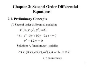
SECOND-ORDER DIFFERENTIAL EQUATIONS 14.1 Second-Order Linear Equations In this section, we will learn how to solve: Homogeneous linear equations for various cases and for initial- and boundary-value problems.
SECOND-ORDER LINEAR EQNS. Equation 1 • A second-order linear differential equationhas the form where P, Q, R, and Gare continuous functions.
SECOND-ORDER LINEAR EQNS. • We saw in Section 9.1 that equations of this type arise in the study of the motion of a spring. • In Section 13.3, we will further pursue this application as well as the application to electric circuits.
HOMOGENEOUS LINEAR EQNS. • In this section, we study the case where G(x) = 0, for all x, in Equation 1. • Such equations are called homogeneouslinear equations.
HOMOGENEOUS LINEAR EQNS. Equation 2 • Thus, the form of a second-order linear homogeneous differential equation is: • If G(x) ≠ 0 for some x, Equation 1 is nonhomogeneousand is discussed in Section 13.2.
SOLVING HOMOGENEOUS EQNS. • Two basic facts enable us to solve homogeneous linear equations. • The first says that, if we know two solutions y1 and y2 of such an equation, then the linear combinationy = c1y1 + c2y2is also a solution.
SOLVING HOMOGENEOUS EQNS. Theorem 3 • If y1(x) and y2(x) are both solutions of the linear homogeneous equation 2 and c1 and c2 are any constants, then the function • y(x) = c1y1(x) + c2y2(x)is also a solution of Equation 2.
SOLVING HOMOGENEOUS EQNS. Proof • Since y1 and y2 are solutions of Equation 2, we have:P(x)y1’’ + Q(x)y1’ + R(x)y1 = 0andP(x)y2’’ + Q(x)y2’ + R(x)y2 = 0
SOLVING HOMOGENEOUS EQNS. Proof • Thus, using the basic rules for differentiation, we have: • P(x)y’’ + Q(x)y’ + R(x)y= P(x)(c1y1 + c2y2)” + Q(x)(c1y1 + c2y2)’ + R(x)(c1y1 + c2y2)
SOLVING HOMOGENEOUS EQNS. Proof • = P(x)(c1y1’’ + c2y2’’) + Q(x)(c1y1’ + c2y2’ ) + R(x)(c1y1 + c2y2) • = c1[P(x)y1’’ + Q(x)y1’ + R(x)y1] + c2[P(x)y2’’ + Q(x)y2’ + R(x)y2]= c1(0) + c2(0) = 0 • Thus, y =c1y1 + c2y2 is a solution of Equation 2.
SOLVING HOMOGENEOUS EQNS. • The other fact we need is given by the following theorem, which is proved in more advanced courses. • It says that the general solution is a linear combination of two linearly independentsolutions y1 and y2.
SOLVING HOMOGENEOUS EQNS. • This means that neither y1 nor y2 is a constant multiple of the other. • For instance, the functions f(x) = x2 and g(x) = 5x2are linearly dependent, but f(x) = ex and g(x) = xexare linearly independent.
SOLVING HOMOGENEOUS EQNS. Theorem 4 • If y1 and y2 are linearly independent solutions of Equation 2, and P(x) is never 0, then the general solution is given by:y(x) = c1y1(x) + c2y2(x)where c1 and c2 are arbitrary constants.
SOLVING HOMOGENEOUS EQNS. • Theorem 4 is very useful because it says that, if we know twoparticular linearly independent solutions, then we know everysolution.
SOLVING HOMOGENEOUS EQNS. • In general, it is not easy to discover particular solutions to a second-order linear equation.
SOLVING HOMOGENEOUS EQNS. Equation 5 • However, it is always possible to do so if the coefficient functions P, Q, and R are constant functions—that is, if the differential equation has the formay’’ + by’ + cy = 0 • where: • a, b, and c are constants. • a ≠ 0.
SOLVING HOMOGENEOUS EQNS. • It’s not hard to think of some likely candidates for particular solutions of Equation 5 if we state the equation verbally. • We are looking for a function y such that a constant times its second derivative y’’ plus another constant times y’ plus a third constant times y is equal to 0.
SOLVING HOMOGENEOUS EQNS. • We know that the exponential function y = erx(where r is a constant) has the property that its derivative is a constant multiple of itself: y’ = rerx • Furthermore, y’’ = r2erx
SOLVING HOMOGENEOUS EQNS. • If we substitute these expressions into Equation 5, we see that y = erxis a solution if: ar2erx +brerx +cerx = 0or (ar2 + br +c)erx = 0
SOLVING HOMOGENEOUS EQNS. Equation 6 • However, erx is never 0. • Thus, y = erx is a solution of Equation 5 if r is a root of the equationar2 + br +c = 0
AUXILIARY EQUATION • Equation 6 is called the auxiliary equation(or characteristic equation) of the differential equation ay’’ + by’ + cy = 0. • Notice that it is an algebraic equation that is obtained from the differential equation by replacing: y’’ by r2, y’ by r, y by 1
FINDING r1 and r2 • Sometimes, the roots r1 and r2of the auxiliary equation can be found by factoring.
FINDING r1 and r2 • In other cases, they are found by using the quadratic formula: • We distinguish three cases according to the sign of the discriminant b2 – 4ac.
CASE I • b2 – 4ac > 0 • The roots r1 and r2 are real and distinct. • So, y1 = er1x and y2 = er2x are two linearly independent solutions of Equation 5. (Note that er2x is not a constant multiple of er1x.) • Thus, by Theorem 4, we have the following fact.
CASE I Solution 8 • If the roots r1 and r2 of the auxiliary equation ar2 + br +c = 0 are real and unequal, then the general solution of ay’’ + by’ +cy = 0 is: y = c1er1x+c2er2x
CASE I Example 1 • Solve the equation y’’ + y’ – 6y = 0 • The auxiliary equation is: r2 + r – 6 = (r – 2)(r + 3) = 0 whose roots are r = 2, –3.
CASE I Example 1 • Thus, by Equation 8, the general solution of the given differential equation is:y =c1e2x +c2e-3x • We could verify that this is indeed a solution by differentiating and substituting into the differential equation.
CASE I • The graphs of the basic solutions f(x) = e2x and g(x) = e–3xof the differential equation in Example 1 are shown in blue and red, respectively. • Some of the other solutions, linear combinations of f and g, are shown in black.
CASE I Example 2 • Solve • To solve the auxiliary equation 3r2 + r – 1 = 0, we use the quadratic formula: • Since the roots are real and distinct, the general solution is:
CASE II • b2 – 4ac = 0 • In this case, r1 = r2. • That is, the roots of the auxiliary equation are real and equal.
CASE II Equation 9 • Let’s denote by r the common value of r1 and r2. • Then, from Equations 7, we have:
CASE II • We know that y1 = erx is one solution of Equation 5. • We now verify that y2 = xerx is also a solution.
CASE II • The first term is 0 by Equations 9. • The second term is 0 because r is a root of the auxiliary equation. • Since y1 = erx and y2 = xerx are linearly independent solutions, Theorem 4 provides us with the general solution.
CASE II Solution 10 • If the auxiliary equation ar2 + br + c = 0 has only one real root r, then the general solution of ay’’ + by’ + cy = 0 is:y =c1erx+ c2xerx
CASE II Example 3 • Solve the equation 4y’’ + 12y’ + 9y = 0 • The auxiliary equation 4r2 + 12r + 9 = 0 can be factored as 2(r + 3)2 = 0. • So, the only root is r = –3/2. • By Solution 10, the general solution is:
CASE II • The figure shows the basic solutions f(x) = e-3x/2 and g(x) = xe-3x/2 in Example 3 and some other members of the family of solutions. • Notice that all of them approach 0 as x→ ∞.
CASE III • b2 – 4ac < 0 • In this case, the roots r1 and r2 of the auxiliary equation are complex numbers. • See Appendix H for information about complex numbers.
CASE III • We can write: r1 = α + iβr2 = α – iβwhere α and β are real numbers. • In fact,
CASE III • Then, using Euler’s equationeiθ = cos θ + i sin θwe write the solution of the differential equation as follows.
CASE III • where c1 = C1 + C2, c2 = i(C1 – C2).
CASE III • This gives all solutions (real or complex) of the differential equation. • The solutions are real when the constants c1 and c2 are real. • We summarize the discussion as follows.
CASE III Solution 11 • If the roots of the auxiliary equation ar2 + br +c = 0 are the complex numbers r1 = α + iβ, r2 = α – iβ, then the general solution of ay’’ + by’ + cy =0 is:y =eαx(c1 cos βx +c2 sin βx)
CASE III Example 4 • Solve the equation y’’ – 6y’ + 13y = 0 • The auxiliary equation is: r2 – 6r + 13 = 0 • By the quadratic formula, the roots are:
CASE III Example 4 • So, by Fact 11, the general solution of the differential equation is: y =e3x(c1 cos 2x +c2 sin 2x)
CASE III • The figure shows the graphs of the solutions in Example 4, f(x) = e3x cos 2x and g(x) = e3x sin 2x, together with some linear combinations. • All solutions approach 0 as x→ -∞.
INITIAL-VALUE PROBLEMS • An initial-value problemfor the second-order Equation 1 or 2 involves finding a solution yof the differential equation that also satisfies initial conditions of the form y(x0) = y0y’(x0) = y1 where y0 and y1 are given constants.