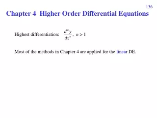
Higher-Order Differential Equations
CHAPTER 3. Higher-Order Differential Equations. (3.1~3.6). Chapter Contents. 3.1 Theory of Linear Equations 3.2 Reduction of Order 3.3 Homogeneous Linear Equations with Constants Coefficients 3.4 Undetermined Coefficients 3.5 Variation of Parameters 3.6 Cauchy-Euler Equations.


Higher-Order Differential Equations
E N D
Presentation Transcript
CHAPTER 3 Higher-Order Differential Equations (3.1~3.6)
Chapter Contents • 3.1 Theory of Linear Equations • 3.2 Reduction of Order • 3.3 Homogeneous Linear Equations with Constants Coefficients • 3.4 Undetermined Coefficients • 3.5 Variation of Parameters • 3.6 Cauchy-Euler Equations
3.1 Preliminary Theory: Linear Equ. • Initial-value ProblemAn nth-order initial problem isSolve: Subject to:(1)with n initial conditions.
Theorem 3.1.1 Existence of a Unique Solution Let an(x), an-1(x), …, a0(x),and g(x)be continuous on I, an(x) 0for all x on I. If x = x0 is any point in this interval, then a solution y(x)of (1) exists on the interval and is unique.
Example 1 Unique Solution of an IVP • The IVP possesses the trivial solution y = 0. Since this DE with constant coefficients, from Theorem 3.1.1, hence y = 0 is the only one solution on any interval containing x = 1.
Example 2 Unique Solution of an VP • Please verify y = 3e2x + e–2x– 3x,is a solution of This DE is linear and the coefficients and g(x)are all continuous, and a2(x) 0 on any I containing x = 0.This DE has an unique solution on I.
Boundary-Value Problem • Solve:Subject to: is called a boundary-value problem (BVP).See Fig 3.1.1.
Example 3 A BVP Can Have Money, Ine, or Not Solutions • In example 4 of Sec 1.1, we see the solution of is x = c1 cos 4t + c2 sin4t (2) (a) Suppose x(0) = 0,then c1 = 0, x(t) = c2 sin 4t Furthermore, x(/2) = 0,we obtain 0 = 0,hence(3)has infinite many solutions. See Fig 3.1.2. (b) If(4)we have c1 = 0, c2= 0, x = 0is the only solution.
Example 3 (2) (c) If (5)we have c1 = 0, and 1 = 0 (contradiction).Hence (5) has no solutions.
Homogeneous Equations • The following DE(6)is said to be homogeneous;(7)with g(x)not identically zero, is nonhomogeneous.
Differential Operators • Let dy/dx = Dy. This symbol D is called a differential operator. We define an nth-order differential operator as (8)In addition, we have(9)so the differential operator L is a linear operator. • Differential EquationsWe can simply write the DEs as L(y) = 0andL(y) = g(x)
Let y1, y2, …, ykbe a solutions of the homogeneous Nth-order differential equation (6) on an interval I. Then the linear combinationy = c1y1(x) + c2y2(x)+ …+ ckyk(x)where the ci, i = 1, 2, …, k are arbitrary constants, is also a solution on the interval. Theorem 3.1.2 Superposition Principles – Homogeneous Equations
Corollaries to Theorem 3.1.2 (a) y = cy1 is also a solution if y1is a solution. (b) A homogeneous linear DE always possesses the trivial solution y = 0.
A set of f1(x), f2(x), …, fn(x)is linearly dependent on an interval I, if there exists constants c1, c2, …, cn, not all zero, such thatc1f1(x) + c2f2(x) + … + cn fn(x) = 0If not linearly dependent, it is linearly independent. Definition 3.1.1 Linear Dependence / Independence Example 4 Superposition – Homogeneous DE • The function y1= x2, y2= x2 ln x are both solutions of Then y = x2+ x2 ln x is also a solution on (0, ).
In other words, if the set is linearly independent,when c1f1(x) + c2f2(x) + … + cn fn(x) = 0then c1 = c2 = … = cn= 0 • Referring to Fig 3.1.3, neither function is a constant multiple of the other, then these two functions are linearly independent. • If two functions are linearly dependent, then one is simply a constant multiple of the other. • Two functions are linearly independent when neither is a constant multiple of the other.
Fig 3.1.3 The set consisting of f1 and f2 is linear independent on (-, )
Example 5 Linear Dependent Functions • The functions f1 = cos2 x, f2 = sin2x, f3 = sec2x, f4 =tan2x are linearly dependent on the interval (-/2, /2) sincec1 cos2 x +c2 sin2x +c3 sec2x +c4 tan2x = 0when c1 = c2 = 1, c3 = -1, c4 = 1.
Example 6 Linearly Dependent Functions • The functions are linearly dependent on the interval (0, ), sincef2 = 1 f1 + 5 f3 + 0 f4
Suppose each of the functions f1(x), f2(x), …, fn(x) possesses at least n – 1 derivatives. The determinantis called the Wronskianof the functions. Definition 3.1.2 Wronskian
Let y1(x), y2(x), …, yn(x) be n solutions of the nth-order homogeneous DE (6) on an interval I. This set of solutions is linearly independent on I if and on if W(y1, y2, …, yn) 0 for every x in the interval. Theorem 3.1.3 Criterion for Linear Independence Solutions
Definition 3.1.3 Fundamental Set of Solutions Any set y1(x), y2(x),… , yn(x) of n linearly independent solutions is said to be a fundamentalset of solutions. There exists a fundamental set of solutions for (6) on an interval I. Theorem 3.1.4 Existence of a Fundamental Set
Let y1(x), y2(x), …, yn(x) be a fundamental set of solutions of homogeneous DE (6) on an interval I. Then the general solution isy = c1y1(x) + c2y2(x) + … + cnyn(x) where ci, i = 1, 2, …, n are arbitrary constants. Theorem 3.1.5 General Solution – Homogeneous Equations
Example 7 General Solution of a Homogeneous DE • The functions y1 = e3x, y2 = e-3xare solutions of y” –9y = 0on (-, )Now for every x. So y = c1e3x + c2e-3xis the general solution.
Example 8 A Solution Obtained from a General Solution • The functions y = 4sinh 3x - 5e3x is a solution of example 7 (Verify it). Observer y = 4 sinh 3x – 5e-3x
Example 9 General Solution of a Homogeneous DE • The functions y1= ex,y2 = e2x , y3 = e3xare solutions of y’’’ –6y” + 11y’ –6y = 0on (-, ). Sincefor everyrealvalueof x. So y = c1ex + c2e2x + c3e3xis the general solution on (-, ).
Any ypfree of parameters satisfying (7) is called a particular solution. If y1(x), y2(x), …, yk(x) be a fundamental set of solutions of (6), then the general solution of (7) isy= c1y1 + c2y2 +… +ckyk + yp(10)where ci, i = 1, 2, …, n are arbitrary constants. Theorem 3.1.6 General Solution – Nonhomogeneous Equations Nonhomogeneous Equations • Complementary Functiony = c1y1 + c2y2 +… +ckyk +yp = yc + yp = complementary + particular
Example 10 General Solution of a Nonhomogeneous DE • The function yp= -(11/12) –½ xis a particular solution of (11)From previous discussions, the general solution of (11) is
Given(12)where i = 1, 2, …, k. If ypi denotes a particular solution corresponding to the DE (12) with gi(x), then(13)is a particular solution of (14) Theorem 3.1.7 Superposition Principles – Nonhomogeneous Equations Any Superposition Principles
Example 11 Superposition – Nonmogeneous DE • We findis a particular solution ofis a particular solution ofis a particular solution of From Theorem 3.1.7, is a solution of
Note • If ypi is a particular solution of (12), then is also a particular solution of (12) when the right-hand member is
3.2 Reduction of Order • IntroductionWe know the general solution of (1)is y = c1y1 + c2y1. Suppose y1(x)denotes a known solution of (1). We assume the other solution y2has the form y2= uy1.Our goal is to find a u(x)and this method is called reduction of order.
Example 1 Finding s second Solution Given y1 = ex is a solution of y” – y = 0,find a second solution y2 by the method of reduction of order. Solution:If y = uex, then And Since ex 0, we let w = u’,then
Example 1 (2) Thus(2)Choosing c1= 0, c2= -2, we have y2= e-x. Because W(ex, e-x) 0for every x, they are independent on (-, ).
General Case • Rewrite (1) as the standard form(3)Let y1(x)denotes a known solution of (3) and y1(x) 0 for every x in the interval. • If we define y = uy1, thenwe have
This implies that or(4)where we let w = u’. Solving (4), we have or
Example 2 A second Solution by Formula (5) The function y1= x2is a solution of Find the general solution on (0, ). Solution:The standard form is From (5)The general solution is
3.3 Homogeneous Linear Equation with Constant Coefficients • Introduction(1)where ai, i = 0, 1, …, n are constants, an 0. • Auxiliary EquationFor n = 2,(2)Try y = emx, then (3)is called an auxiliary equation.
From (3) the two roots are(1) b2 – 4ac > 0: two distinct real numbers.(2) b2 – 4ac = 0: two equal real numbers.(3) b2 – 4ac < 0: two conjugate complex numbers.
Case 1: Distinct real rootsThe general solution is(4) • Case 2: Repeated real rootsand from (5) of Sec 3.2, (5)The general solution is (6)
Case 3: Conjugate complex rootsWe write , a general solution is From Euler’s formula: and(7) and
Sinceis a solution then setC1= C1 = 1and C1 = 1, C2 = -1 , we have two solutions: So, ex cos x and exsin x are a fundamental set of solutions, that is, the general solution is(8)
Example 1 Second-Order DEs • Solve the following DEs: (a) (b) (c)
Example 2 An Initial-Value Problem Solve Solution:See Fig 3.3.1.
Two Equations worth Knowing • For the first equation:(9)For the second equation:(10)Let Then(11)
Higher-Order Equations • Given (12)we have(13)as an auxiliary equation. • If the roots of (13) are real and distinct, then the general solution of (12) is
Example 3 Third-Order DE Solve Solution: