Download
1 / 33
330 likes | 360 Vues
Explore the concepts of metaball modeling and polygonalization in advanced graphics, including force functions, octrees, and the marching cubes algorithm.

E N D
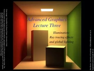
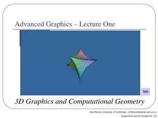
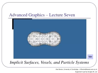
Advanced Graphics – Lecture Seven Implicit Surfaces, Voxels, and Particle Systems Alex Benton, University of Cambridge – A.Benton@damtp.cam.ac.uk Supported in part by Google UK, Ltd
Blobby modeling • “Metaball, or ‘Blobby’, Modeling is a technique which uses implicit surfaces to produce models which seem more ‘organic’ or ‘blobby’ than conventional models built from flat planes and rigid angles”. --me • Uses of blobby modelling: • Organic forms and nonlinear shapes • Scientific modelling (electron orbitals, some medical imaging) • Muscles and joints with skin • Rapid prototyping • CAD/CAM solid geometry
“New Train” - Wyvill Blobby modeling examples-- Paul Bourke (1997) “Cabrit Model” - Wyvill
How it works • The user controls a set of control points instead of working directly with the surface. The control points in turn influence the shape of the model. • Each point in space generates a field of force, which drops off as a function of distance from the point; ex: gravity weakening with distance. • A blobby model is formed from the shells of these force fields, the implicit surface which they define in space. • An implicit surface is a surface consisting of all the points in space where a mathematical function (in this case, the value of the force field) has a particular key value (such as 0.5). Force = 2 1 0.5 0.25 ...
Force functions • Several force functions work well. Examples: • “Blobby Molecules” – Jim Blinn • F(r) = a e-br2 • Here ‘b’ is related to the standard deviation of the curve, and ‘a’ to the height. • “Metaballs” – Jim Blinn a(1- 3r2 / b2) 0 ≤ r < b/3 F(r) = (3a/2)(1-r/b)2 b/3 ≤ r < b 0 b ≤ r • Here ‘a’ is a scaling factor and ‘b’ bounds the radius of effect
Force functions • “Soft Objects” – Wyvill & Wyvill • F(r) = a(1 - 4r6/9b6 + 17r4/9b4 - 22r2 / 9b2) • This is the first few terms in the series expansion of an exponential function. • Here ‘a’ scales the function and ‘b’ sets radius of influence. • Advantage : rapid computation.
Finding the surface • An octree is a recursive subdivision of space which “homes in” on the surface, from larger to finer detail. • An octree encloses a cubical volume in space. You evaluate the force function F(r) at each vertex of the cube. • As the octree subdivides and splits into smaller octrees, only the octrees which contain some of the surface are processed; empty octrees are discarded.
Polygonalizing the surface • To display a set of octrees, convert the octrees into polygons. • Each corner of each octree has a value for the force function. • If some corners are “hot” (above the force limit) and others are “cold” (below the force limit) then the implicit surface crosses the cube edges in between. • The set of midpoints of adjacent crossed edges forms one or more rings, which can be triangulated. The normal is known from the hot/cold direction on the edges. • To refine the polygonalization, subdivide recursively; discard any child whose vertices are all hot or all cold.
Polygonalizing the surface • Recursive subdivision :
Polygonalizing the surface • There are fifteen possible configurations (up to symmetry) of hot/cold vertices in the cube. → • With rotations, that’s 256 cases. • Beware: there are ambiguous cases in the polygonalization which must be addressed separately. ↓ Images courtesy of Diane Lingrand
Polygonalizing the surface • One way to overcome the ambiguities that arise from the cube is to decompose the cube into tretrahedra. • A common decomposition is into five tetrahedra. → • Caveat: need to flip every other cube. (Why?) • Can also split into six. • Another way is to do the subdivision itself on tetrahedra—no cubes at all. Image from the Open Problem Garden
Smoothing the surface • Improved edge vertices • The naïve implementation builds polygons whose vertices are the midpoints of the edges which lie between hot and cold vertices. • The vertices of the implicit surface can be more closely approximated by points linearly interpolated along the edges of the cube by the weights of the relative values of the force function. • t = (0.5 - F(P1)) / (F(P2) - F(P1)) • P = P1 + t (P2 - P1)
Marching cubes • An alternative to octrees if you only want to compute the final stage is the marching cubes algorithm (Lorensen & Cline, 1985): • Fire a ray from any point known to be inside the surface. • Using Newton’s method or binary search, find where the ray crosses the surface. • Newton: derivative estimated from discrete local sampling • There may be many crossings • Drop a cube around the intersection point: it will have some vertices hot, some cold. • While there exists a cube which has at least one hot vertex and at least one cold vertex on a side and no neighbor on that side, create a neighboring cube on that side. Repeat. Marching cubes is common in medical imaging such as MRI scans. It was first demonstrated (and patented!) by researchers at GE in 1984, modeling a human spine.
Pros and cons of blobby modelling • Benefits: • Very rapid general shapes • Allows rapid manipulation at multiple levels of detail • Surface complexity is not a function of data complexity • Enables a “poor man’s” solid geometry • Downsides: • Flat surfaces, sharp angles, etc. are difficult • Difficult to precisely achieve targeted features • “Popping” between octree levels can be misleading
Blobby modelling—what else? • Complex primitives • Why settle for a point when you could have a line, or a spline, or a weather system from NASA? • Colors and textures • The same math that blends forces can blend colors and textures as well • Editing textures on an implicit surface is an ongoing topic of research—edits that survive animation are tricky
Voxels and volume rendering • A voxel (“volume pixel”) is a cube in space with a given color; like a 3D pixel. • Voxels are often used for medical imaging, terrain, scanning and model reconstruction, and other very large datasets. • Voxels usually contain color but could contain other data as well—flow rates (in medical imaging), density functions (analogous to implicit surface modeling), lighting data, surface normals, 3D texture coordinates, etc. • Often the goal is to render the voxel data directly, not to polygonalize it.
Volume ray casting If speed can be sacrificed for accuracy, render voxels with volume ray casting: • Fire a ray through each pixel; • Sample the voxel data along the ray, computing the weighted average (trilinear filter) of the contributions to the ray of each voxel it passes through or near; • Compute surface gradient from of each voxel from local sampling; generate surface normals; compute lighting with the standard lighting equation; • ‘Paint’ the ray from back to front, occluding more distant voxels with nearer voxels; this gives hidden-surface removal and easy support for transparency. The steps of volume rendering; a volume ray-cast skull. Images from wikipedia.
Sampling in voxel rendering • Why trilinear filtering? • If we just show the color of the voxel we hit, we’ll see the exact edges of every cube. • Instead, choose the weighted average between adjacent voxels. • Trilinear: averaging across X, Y, and Z Your sample will fall somewhere between eight (in 3d) voxel centers. Weight the color of the sample by the inverse of its distance from the center of each voxel.
Reasonably fast voxels • If speed is of the essence, cast your rays but stop at the first opaque voxel. • Store precomputed lighting directly in the voxel • Works for diffuse and ambient but not specular • Popular technique for video games (e.g. Comanche →) • Another clever trick: store voxels in a sparse voxel octree. • Watch for it in id’s next-generation engine… Comanche Gold, NovaLogic Inc (1998) Sparse Voxel Octree Ray-Casting, Cyril Crassin
If speed is essential (like if, say, you’re writing a video game in 1992) and you know that your terrain can be represented as a height-map (ie., without overhangs), replace ray-casting with ‘column’-casting and use a “Y-buffer”: Draw from front to back, drawing columns of pixels from the bottom of the screen up. For each pixel in receding order, track the current max y height painted and only draw new pixels above that y. Anything shorter must be behind something that’s nearer, and it’s shorter; so don’t draw it. Ludicrously fast voxels D e p t h Depth
Particle systems • Particle systems are a monte-carlo style technique which uses thousands (or millions) or tiny graphical artefacts to create large-scale visual effects. • Particle systems are used for hair, fire, smoke, water, clouds, explosions, energy glows, in-game special effects and much more. • The basic idea:“If lots of little dots all do something the same way, our brains will see the thing they do and not the dots doing it.” A particle system created with 3dengfx, from wikipedia. Screenshot from the game Command and Conquer 3 (2007) by Electronic Arts; the “lasers” are particle effects.
History of particle systems • 1962: Ships explode into pixel clouds in “Spacewar!”, the 2nd video game ever. • 1978: Ships explode into broken lines in “Asteroid”. • 1982: The Genesis Effect in “Star Trek II: The Wrath of Khan”. Fanboy note: OMG. You can play the original Spacewar! at http://spacewar.oversigma.com/ -- the actual original game, running in a PDP-1emulator inside a Java applet.
“The Genesis Effect” – William ReevesStar Trek II: The Wrath of Khan (1982)
Particle systems • How it works: • Particles are generated from an emitter. • Emitter position and orientation are specified discretely; • Emitter rate, direction, flow, etc are often specified as a bounded random range (monte carlo) • Time ticks; at each tick, particles move. • New particles are generated; expired particles are deleted • Forces (gravity, wind, etc) accelerate each particle • Acceleration changes velocity • Velocity changes position • Particles are rendered.
Particle systems — emission • Each frame, your emitter will generate new particles. • Here you have two choices: • Constrain the average number of particles generated per frame: • # new particles = average # particles per frame + rand() variance • Constrain the average number of particles per screen area: • # new particles = average # particles per area + rand() variance screen area Transient vs persistent particles emitted to create a ‘hair’ effect (source: Wikipedia)
Each new particle will have at least the following attributes: initial position initial velocity (speed and direction) You now have a choice of integration technique: Evaluate the particles at arbitrary time t as a closed-form equation for a stateless system. Or, use iterative (numerical) integration: Euler integration Verlet integration Runge-Kutta integration Particle systems — integration
Closed-form function: Represent every particle as a parametric equation; store only the initial position p0, initial velocity v0, and some fixed acceleration (such as gravity g.) p(t)=p0+v0t+½gt2 No storage of state Very limited possibility of interaction Best for water, projectiles, etc—non-responsive particles. Discrete integration: Remember your physics—integrate acceleration to get velocity: v’=v + a •∆t Integrate velocity to get position: p’=p + v •∆t Collapse the two, integrate acceleration to position: p’’=2p’-p + a •∆t2 Timestep must be nigh-constant; collisions are hard. Particle systems — two integration shortcuts:
Particle systems—rendering • Can render particles as points, textured polys, or primitive geometry • Minimize the data sent down the pipe! • Polygons with alpha-blended images make pretty good fire, smoke, etc • Transitioning one particle type to another creates realistic interactive effects • Ex: a ‘rain’ particle becomes an emitter for ‘splash’ particles on impact • Particles can be the force sources for a blobby model implicit surface • This is an effective way to simulate liquids Images by nvidia
References Blobby modelling: • D. Ricci, A Constructive Geometry for Computer Graphics, Computer Journal, May 1973 • J Bloomenthal, Polygonization of Implicit Surfaces, Computer Aided Geometric Design, Issue 5, 1988 • B Wyvill, C McPheeters, G Wyvill, Soft Objects, Advanced Computer Graphics (Proc. CG Tokyo 1986) • B Wyvill, C McPheeters, G Wyvill, Animating Soft Objects, The Visual Computer, Issue 4 1986 • http://astronomy.swin.edu.au/~pbourke/modelling/implicitsurf/ • http://www.cs.berkeley.edu/~job/Papers/turk-2002-MIS.pdf • http://www.unchainedgeometry.com/jbloom/papers/interactive.pdf • http://www-courses.cs.uiuc.edu/~cs319/polygonization.pdf Voxels: • J. Wilhelms and A. Van Gelder, A Coherent Projection Approach for Direct Volume Rendering, Computer Graphics, 35(4):275-284,July 1991. • http://en.wikipedia.org/wiki/Volume_ray_casting Particle Systems: • William T. Reeves, “Particle Systems - A Technique for Modeling a Class of Fuzzy Objects”, Computer Graphics 17:3 pp. 359-376, 1983 (SIGGRAPH 83). • Lutz Latta, Building a Million Particle System, http://www.2ld.de/gdc2004/MegaParticlesPaper.pdf , 2004 • http://en.wikipedia.org/wiki/Particle_system