Download
1 / 36
380 likes | 1.18k Vues
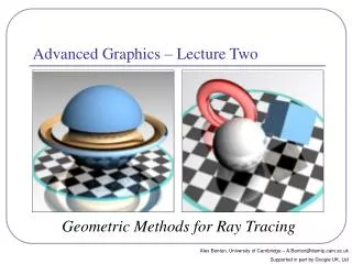
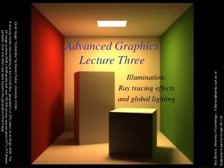
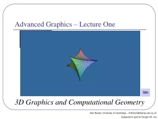
Advanced Graphics Lecture Three Cover image: “ Cornell Box” by Steven Parker, University of Utah.

E N D
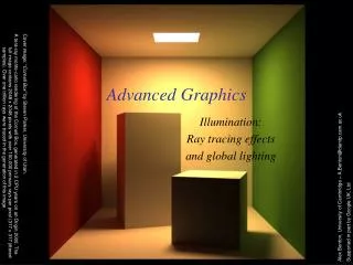
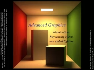
Advanced GraphicsLecture Three Cover image: “Cornell Box” by Steven Parker, University of Utah. A tera-ray monte-carlo rendering of the Cornell Box, generated in 2 CPU years on an Origin 2000. The full image contains 2048 x 2048 pixels with over 100,000 primary rays per pixel (317 x 317 jittered samples). Over one trillion rays were traced in the generation of this image. Illumination: Ray tracing effects and global lighting Alex Benton, University of Cambridge – A.Benton@damtp.cam.ac.uk Supported in part by Google UK, Ltd
Lighting revisited • We approximate lighting as the sum of the ambient, diffuse, and specular components of the light reflected to the eye. • Associate scalar parameters kA, kDand kS with the surface. • Calculate diffuse and specularfrom each light source separately. L1 L2 R N P D O
Lighting revisited—ambient lighting • Ambient light is a flat scalar constant, LA. • The amount of ambient light LA is a parameter of the scene; the way it illuminates a particular surface is a parameter of the surface. • Some surfaces (ex: cotton wool) have high ambient coefficient kA; others (ex: steel tabletop) have low kA. • Lighting intensity for ambient light alone:
Lighting revisited—diffuse lighting • The diffuse coefficient kD measures how much light scatters off the surface. • Some surfaces (e.g. skin) have high kD, scattering light from many microscopic facets and breaks. Others (e.g. ball bearings) have low kD. • Diffuse lighting intensity: L N N θ L
Lighting revisited—specular lighting • The specular coefficient kS measures how much light reflects off the surface. • A ball bearing has high kS; I don’t. • ‘Shininess’ is approximated by a scalar power n. • Specular lighting intensity: E N L α R
Lighting revisited—all together • The total illumination at P is therefore: E N θ L α R
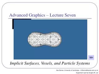
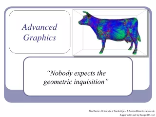
Ambient=1 Diffuse=0 Specular=0 Ambient=0 Diffuse=1 Specular=0 Ambient=0.2 Diffuse=0.4 Specular=0.4 (n=2) Ambient=0 Diffuse=0 Specular=1 (n=2)
Spotlights • To create a spotlight shining along axis S, you can multiply the (diffuse+specular) term by (max(L•S,0))m. • Raising m will tighten the spotlight,but leave the edges soft. • If you’d prefer a hard-edged spotlightof uniform internal intensity, you can use a conditional, e.g.((L•S > cos(15˚)) ? 1 : 0). S θ L P D O
Ray tracing—Shadows • To simulate shadow in ray tracing, fire a ray from P towards each light Li. If the ray hits another object before the light, then discard Li in the sum. • This is a boolean removal, so itwill give hard-edged shadows. • Hard-edged shadows imply apinpoint light source.
Softer shadows • Shadows in nature are not sharp because light sources are not infinitely small. • Also because light scatters, etc. • For lights with volume, fire many rays, covering the cross-section of your illuminated space. • Illumination is (the total number of raysthat aren’t blocked) divided by (the totalnumber of rays fired). • This is an example of Monte-Carlo integration: a coarse simulation of an integral over a space by randomly sampling it with many rays. • The more rays fired, the smoother the result. L1 P D O
Reflection • Reflection rays are calculated by: R = 2(-D•N)N+D …just like the specular reflection ray. • Finding the reflected color is a recursive raycast. • Reflection has scene-dependant performance impact. L1 Q P D O
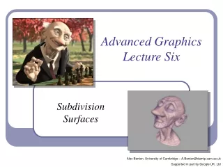
num bounces=0 num bounces=2 num bounces=1 num bounces=3
Transparency • To add transparency, generate and trace a new transparency ray with OT=P, DT=D. • Option 1 (object state): • Associate a transparency value A with the material of the surface, like reflection. • Option 2 (RGBA): • Make color a 1x4 vector where the fourth component, ‘alpha’, determines the weight of the recursed transparency ray.
Refraction • Snell’s Law: “The ratio of the sines of the angles of incidence of a ray of light at the interface between two materials is equal to the inverse ratio of the refractive indices of the materials is equal to the ratio of the speeds of light in the materials.” Historical note: this formula has been attributed to Willebrord Snell (1591-1626) and Rene’ Descartes (1596-1650) but first discovery goes to Ibn Sahl (940-1000) of Baghdad.
Refraction • The angle of incidence of a ray of light where it strikes a surface is the acute angle between the ray and the surface normal. • The refractive index of a material is a measure of how much the speed of light1 is reduced inside the material. • The refractive index of air is about 1.003. • The refractive index of water is about 1.33. 1 Or sound waves or other waves
Refraction in ray tracing • Using Snell’s Law and the angle of incidence of the incoming ray, we can calculate the angle from the negative normal to the outbound ray. P’ N θ2 P θ1 D O
Refraction in ray tracing • What if the arcsin parameter is > 1? • Remember, arcsin is defined in [-1,1]. • We call this the angle of total internal reflection, where the light becomes trapped completely inside the surface. Total internal reflection P’ N θ2 P θ1 D O
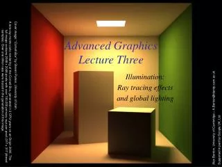
Refractive index vs transparency 0.25 0.5 0.75 t=1.0 n = 1.0 1.1 1.2 1.3 1.4 1.5
What’s wrong with raytracing? • Soft shadows are expensive • Shadows of transparent objects require further coding or hacks • Lighting off reflective objects follows different shadow rules from normal lighting • Hard to implement diffuse reflection (color bleeding, such as in the Cornell Box—notice how the sides of the inner cubes are shaded red and green.) • Fundamentally, the ambient term is a hack and the diffuse term is only one step in what should be a recursive, self-reinforcing series. The Cornell Box is a test for rendering Software, developed at Cornell University in 1984 by Don Greenberg. An actual box is built and photographed; an identical scene is then rendered in software and the two images are compared.
Radiosity • Radiosity is an illumination method which simulates the global dispersion and reflection of diffuse light. • First developed for describing spectral heat transfer (1950s) • Adapted to graphics in the 1980s at Cornell University • Radiosity is a finite-element approach to global illumination: it breaks the scene into many small elements (‘patches’) and calculates the energy transfer between them. Images from Cornell University’s graphics group http://www.graphics.cornell.edu/online/research/
Radiosity—algorithm • Surfaces in the scene are divided into form factors (also called patches), small subsections of each polygon or object. • For every pair of form factors A, B, compute a view factor describing how much energy from patch A reaches patch B. • The further apart two patches are in space or orientation, the less light they shed on each other, giving lower view factors. • Calculate the lighting of all directly-lit patches. • Bounce the light from all lit patches to all those they light, carrying more light to patches with higher relative view factors. Repeating this step will distribute the total light across the scene, producing a total illumination model. Note: very unfortunately, some literature uses the term ‘form factor’ for the view factor as well.
Radiosity—mathematical support • The ‘radiosity’ of a single patch is the amount of energy leaving the patch per discrete time interval. • This energy is the total light being emitted directly from the patch combined with the total light being reflected by the patch: where… • Bi is the radiosity of patch i; Bj is the cumulative radiosity of all other patches (j≠i) • Ei is the emitted energy of the patch • Ri is the reflectivity of the patch • Fij is the view factor of energy from patch i to patch j.
Radiosity—form factors • Finding form factors can be done procedurally or dynamically • Can subdivide every surface into small patches of similar size • Can dynamically subdivide wherever the 1st derivative of calculated intensity rises above some threshold. • Computing cost for a general radiosity solution goes up as the square of the number of patches, so try to keep patches down. • Subdividing a large flat white wall could be a waste. • Patches should ideally closely align with lines of shadow.
Radiosity—implementation (A) Simple patch triangulation (B) Adaptive patch generation: the floor and walls of the room are dynamically subdivided to produce more patches where shadow detail is higher. Images from “Automatic generation of node spacing function”, IBM (1998) http://www.trl.ibm.com/ projects/meshing/nsp/nspE.htm (A) (B)
One equation for the view factor between patches i, j is: …where θi is the angle between the normal of patch i and the line to patch j, r is the distance and V(i,j) is the visibility from i to j (0 for occluded, 1 for clear line of sight.) Radiosity—view factors High view factor θj θi Low view factor
Calculating V(i,j) can be slow. One method is the hemicube, in which each form factor is encased in a half-cube. The scene is then ‘rendered’ from the point of view of the patch, through the walls of the hemicube; V(i,j) is computed for each patch based on which patches it can see (and at what percentage) in its hemicube. A purer method, but more computationally expensive, uses hemispheres. Radiosity—calculating visibility Note: This method can be accelerated using modern graphics hardware to render the scene. The scene is ‘rendered’ with flat lighting, setting the ‘color’ of each object to be a pointer to the object in memory.
Radiosity gallery Image from GPU Gems II, nVidia Teapot (wikipedia) Image from A Two Pass Solution to the Rendering Equation: a Synthesis of Ray Tracing and Radiosity Methods, John R. Wallace, Michael F. Cohen and Donald P. Greenberg (Cornell University, 1987)
Shadows, refraction and caustics • Problem: shadow ray strikes transparent, refractive object. • Refracted shadow ray will now miss the light. • This destroys the validity of the boolean shadow test. • Problem: light passing through a refractive object will sometimes form caustics (right), artifacts where the envelope of a collection of rays falling on the surface is bright enough to be visible. This is a photo of a real pepper-shaker. Note the caustics to the left of the shaker, in and outside of its shadow. Photo credit: Jan Zankowski
Shadows, refraction and caustics • Solutions for shadows of transparent objects: • Backwards ray tracing (Arvo) • Very computationally heavy • Improved by stencil mapping (Shenya et al) • Shadow attenuation (Pierce) • Low refraction, no caustics • More general solution: • Photon mapping (Jensen)→ Image from http://graphics.ucsd.edu/~henrik/ Generated with photon mapping
Photon mapping • Photon mapping is the process of emitting photons into a scene and tracing their paths probabilistically to build a photon map, a data structure which describes the illumination of the scene independently of its geometry. This data is then combined with ray tracing to compute the global illumination of the scene. Image by Henrik Jensen (2000)
Photon mapping—algorithm (1/2) Photon mapping is a two-pass algorithm: 1. Photon scattering • Photons are fired from each light source, scattered in randomly-chosen directions. The number of photons per light is a function of its surface area and brightness. • Photons fire through the scene (re-use that raytracer, folks.) Where they strike a surface they are either absorbed, reflected or refracted. • Wherever energy is absorbed, cache the location, direction and energy of the photon in the photon map. The photon map data structure must support fast insertion and fast nearest-neighbor lookup; a kd-tree1 is often used. Image by Zack Waters 1 A kd-tree is a type of binary space partitioning tree. Space is recursively subdivided by axis-aligned planes and points on either side of each plane are separated in the tree. The kd-tree has O(n log n) insertion time (but this is very optimizable by domain knowledge) and O(n2/3) search time.
Photon mapping—algorithm (2/2) Photon mapping is a two-pass algorithm: 2. Rendering • Ray trace the scene from the point of view of the camera. • For each first contact point P use the ray tracer for specular but compute diffuse from the photon map and do away with ambient completely. • Compute radiant illumination by summing the contribution along the eye ray of all photons within a sphere of radius r of P. • Caustics can be calculated directly here from the photon map. For speed, the caustic map is usually distinct from the radiance map. Image by Zack Waters
Photon mapping—a few comments • This method is a great example of Monte Carlo integration, in which a difficult integral (the lighting equation) is simulated by randomly sampling values from within the integral’s domain until enough samples average out to about the right answer. • This means that you’re going to be firing millions of photons. Your data structure is going to have to be very space-efficient. http://www.okino.com/conv/imp_jt.htm
0 pd ps pt 1 Photon mapping—a few comments • Initial photon direction is random. Constrained by light shape, but random. • What exactly happens each time a photon hits a solid also has a random component: • Based on the diffuse reflectance, specular reflectance and transparency of the surface, compute probabilities pd, psand pt where (pd+ps+pt)≤1. This gives a probability map: • Choose a random value p є [0,1]. Where p falls in the probability map of the surface determines whether the photon is reflected, refracted or absorbed. This surface would have minimal specular highlight.
Photon mapping gallery http://graphics.ucsd.edu/~henrik/images/global.html http://web.cs.wpi.edu/~emmanuel/courses/cs563/write_ups/zackw/photon_mapping/PhotonMapping.html http://www.pbrt.org/gallery.php
References Ray tracing| • Foley & van Dam, Computer Graphics (1995) • Jon Genetti and Dan Gordon, Ray Tracing With Adaptive Supersampling in Object Space, http://www.cs.uaf.edu/~genetti/Research/Papers/GI93/GI.html (1993) • Zack Waters, “Realistic Raytracing”, http://web.cs.wpi.edu/~emmanuel/courses/cs563/write_ups/zackw/realistic_raytracing.html Radiosity • nVidia: http://http.developer.nvidia.com/GPUGems2/gpugems2_chapter39.html • Cornell: http://www.graphics.cornell.edu/online/research/ • Wallace, J. R., K. A. Elmquist, and E. A. Haines. 1989, “A Ray Tracing Algorithm for Progressive Radiosity.” In Computer Graphics (Proceedings of SIGGRAPH 89) 23(4), pp. 315–324. • Buss, “3-D Computer Graphics: A Mathematical Introduction with OpenGL” (Chapter XI), Cambridge University Press (2003) Photon mapping • Henrik Jenson, “Global Illumination using Photon Maps”, http://graphics.ucsd.edu/~henrik/ • Zack Waters, “Photon Mapping”, http://web.cs.wpi.edu/~emmanuel/courses/cs563/write_ups/zackw/photon_mapping/PhotonMapping.html