Advanced Graphics
This presentation delves into querying geometric properties like normals at vertices, curvature, convex hull, bounding box, and center of mass on polygonal models. It explores finding normals using the limit definition, weighted averages, and face angles. Discussions include Gaussian curvature on smooth and discrete surfaces, angle deficit at vertices, and the Poincaré Formula for Euler Characteristic. A comprehensive study for geometry enthusiasts and researchers.

Advanced Graphics
E N D
Presentation Transcript
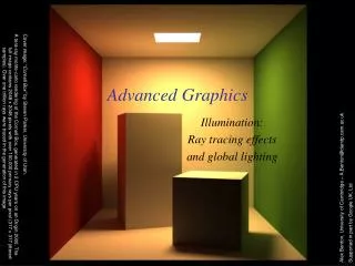
Advanced Graphics “Nobody expects the geometric inquisition” Alex Benton, University of Cambridge – A.Benton@damtp.cam.ac.uk Supported in part by Google UK, Ltd
Querying your geometry • Given a polygonal model, how might you find… • the normal at each vertex? • the curvature at each vertex? • the convex hull? • the bounding box? • the center of mass?
Querying your geometry • A recurring theme here will be, “The polygons are not the shape: the polygons approximate the surface of the shape.” • Some questions from past lectures (e.g. ray-polygon intersection) were about the actual polygons. • But other questions, like the normal at a vertex, are really about approximating the underlying surface as closely as possible.
Normal at a vertex • Expressed as a limit, The normal of surface S at point P is the limit of the cross-product between two (non-collinear) vectors from P to the set of points in S at a distance r from P as r goes to zero. [Excluding orientation.]
Normal at a vertex • Using the limit definition, is the ‘normal’ to a discrete surface necessarily a vector? • The normal to the surface at any point on a face is a constant vector. • The ‘normal’ to the surface at any edge is an arc swept out on a unit sphere between the two normals of the two faces. • The ‘normal’ to the surface at a vertex is a space swept out on the unit sphere between the normals of all of the adjacent faces.
Method 1: Take the average of the normals of surrounding polygons Problem: splitting one adjacent face into 10,000 shards would skew the average Finding the normal at a vertex
Method 2: Take the weighted average of the normals of surrounding polygons, weighted by the area of each face 2a: Weight each face normal by the area of the face divided by the total number of vertices in the face Problem: Introducing new edges into a neighboring face (and thereby reducing its area) should not change the normal. Should making a face larger affect the normal to the surface near its corners? Argument for yes: If the vertices interpolate the ‘true’ surface, then stretching the surface at a distance could still change the local normals. Finding the normal at a vertex
Method 3: Take the weighted average of the normals of surrounding polygons, weighted by each polygon’s face angle at the vertex Face angle: the angle αformed at the vertex v by the vectors to the next and previous vertices in the face F Finding the normal at a vertex Note: In this equation, arccos implies a convex polygon. Why?
Gaussian curvature on smooth surfaces • Informally speaking, the curvature of a surface expresses “how flat the surface isn’t”. • One can measure the directions in which the surface is curving most; these are the directions of principal curvature, k1and k2. • The product of k1and k2 is the scalar Gaussian curvature. Image by Eric Gaba, from Wikipedia
anus 0 on a plane as anus r-2 on a sphere of radius r as (please pretend that this is a sphere) Gaussian curvature on smooth surfaces • Formally, the Gaussian curvature of a region on a surface is the ratio between the area of the unit sphere swept out by the normals of that region and the area of the region itself. • The Gaussian curvature of a point is the limit of this ratio as the region tends to zero area. Area of the projections of the normals on the unit sphere Area on the surface
Gaussian curvature on discrete surfaces • On a discrete surface, normals do not vary smoothly: the normal to a face is constant on the face, and at edges and vertices the normal is—strictly speaking—undefined. • Normals change instantaneously (as one's point of view travels across an edge from one face to another) or not at all (as one's point of view travels within a face.) • The Gaussian curvature of the surface of any polyhedral mesh is zero everywhere except at the vertices, where it is infinite.
Angle deficit – a better solution for measuring discrete curvature • The angle deficitAD(v) of a vertex v is defined to be two π minus the sum of the face angles of the adjacent faces. AD(v) = 360 ˚ – 270 ˚ = 90 ˚ 90˚ 90˚ 90˚
Angle deficit High angle deficit Low angle deficit Negative angle deficit
Angle deficit Hmmm…
Genus, Poincaré and the Euler Characteristic • Formally, the genus g of a closed surface is ...“a topologically invariant property of a surface defined as the largest number of nonintersecting simple closed curves that can be drawn on the surface without separating it.” --mathworld.com • Informally, it’s the number of coffee cup handles in the surface. Genus 0 Genus 1
Genus, Poincaré and the Euler Characteristic • Given a polyhedral surface S without border where: • V = the number of vertices of S, • E = the number of edges between those vertices, • F = the number of faces between those edges, • χ is the Euler Characteristic of the surface, the Poincaré Formula states that:
Genus, Poincaré and the Euler Characteristic 4 faces 3 faces g = 1 E = 24 F = 12 V = 12 V-E+F = 2-2g = 0 g = 0 E = 12 F = 6 V = 8 V-E+F = 2-2g = 2 g = 0 E = 15 F = 7 V = 10 V-E+F = 2-2g = 2
The Euler Characteristic and angle deficit • Descartes’ Theorem of Total Angle Deficit states that on a surface S with Euler characteristic χ, the sum of the angle deficits of the vertices is2πχ: • Cube: • χ = 2-2g = 2 • AD(v) = π/2 • 8(π/2) = 4π = 2πχ • Tetrahedron: • χ = 2-2g = 2 • AD(v) = π • 4(π) = 4π = 2πχ
Convex hull • The convex hull of a set of points is the unique surface of least area which contains the set. • If a set of infinite half-planes have a finite non-empty intersection, then the surface of their intersection is a convex polyhedron. • If a polyhedron is convex then for any two faces A and B in the polyhedron, all points in B which are not in A lie to the same side of the plane containing A. • Every point on a convex hull has non-negative angle deficit. • The faces of a convex hull are always convex.
Method 1: For every triple of points in the set, define a plane P. If all other points in the set lie to the same side of P (dot-product test) then add P to the hull; else discard. Problem 1: this works but it’s O(n4). Finding the convex hull of a set of points
Finding the convex hull of a set of points • Method 2: • Initialize C with a tetrahedron from any four non-colinear points in the set. Orient the faces of C by taking the dot product of the center of each face with the average of the vertices of C. • For each vertex v, • For each face f of C, • If the dot product of the normal of f with the vector from the center of f to v is positive then v is ‘above’ f. • If v is above f then delete f and update a (sorted) list of all new border vertices. • Create a new triangular face from v to each pair of border vertices. • Problem 2: • This is O(n2) at best.
Finding the convex hull of a set of points Method 3: • The exterior boundary of the union of the cells of the Delaunay triangulation of a set of points is its convex hull. • Algorithm: • Find the Voronoi diagram of your point set • Compute the Delaunay triangulation (2D) or tetrahedralization (3D) • Delete all faces of the simplices which aren’t on the exterior border The exterior border of the Delaunay triangulation is the convex hull of the point set.
Testing if a point is inside a convex hull • We can generalize Method 2 to test whether a point is inside any convex polyhedron. • For each face, test the dot product of the normal of the face with a vector from the face to the point. If the dot is ever positive, the point lies outside. • The same logic applies if you’re storing normals at vertices.
Bounding volumes • Bounding boxes help to quickly accelerate volumetric tests, such as “does the laser hit the cow?” • Works great with scene graphs • For many applications, bboxes don’t have to be tight • Often choose fast hit testing over accuracy • Axis-aligned bounding boxes • max and min of x/y/z. • Bounding spheres • Max of radius from some rough center • Bounding cylinders • Common in early FPS games
Minimal bounding circle • The minimum bounding circle of a set of points in a plane: • Let C be a circle of radius r enclosing all points. • Let a be the point farthest from the center of C. Shrink r until C touches a. • Move the center of C towards a and shrink r until a second point b lies on C. • If (|a-b| < 2r)then: • Shrink r until C touches a third point, e. • If e lies on the opposite hemicircle from a and b, done. • Else redefine a, b as the two furthest points of {a,b,e} and repeat. • This can clearly be generalized to three dimensions. • This algorithm is O(n2). Nimrod Meggido (1983) has given a more complicated—but linear-time—algorithm.
Oriented bounding boxes (OBBs) • Bounding spheres are rarely optimal. • Axis-aligned bounding boxes are also suboptimal; oriented bounding boxes will fit tighter. • OBBs are not quite so fast to test as AABBs but they have fewer false positives. • Joe O’Rourke (1985) gives an O(n3) algorithm for finding oriented bounding boxes.
Centroids • The centroid of a surface is the center of mass of the volume enclosed by the surface. • This is not the same as the center of the bounding box. • We’ll assume that the ‘material’ within the surface is of uniform density. • We’ll also assume that we have a closed surface (without border.)
Centroids • Method 1: Take the average of all vertices. C = (Σ{v}(v)) / ||{v}|| • Problem 1: as with normals, an area of bizarre density would skew the average. True centroid Average of vertices ~50 verts ~500 verts Center of bounding box
Centroids • Method 2: Take the average of the centers of the faces of the surface, weighting each by the area of the face. • This method works well for convex polyhedra. • Problem 2: This is vulnerable to dense ‘wrinkles’ of many polygons packed into a small volume. The average adult human brain has a surface area of approximately 2,500 cm2, a volume of roughly 1200 cm3, and weighs about 1400g. By comparison, a sphere of similar volume would have a surface area of 546 cm2. Brain image courtesy of Moprhonix.com.
Method 3a: Use “Monte Carlo” integration. Find the bounding box of the surface and then choose billions of points at random inside the box; take the average of all those points which fall inside the surface. Problem 3a: Testing for ‘inside’ is time-consuming (although it can be accelerated; try BSP trees.) Also, this lacks precision. And, frankly, finesse. Method 3b: Decompose the polyhedron into convex polyhedra, then use method 2 to find the center of each. Average the centers, weighting each point by the volume of its convex polyhedron. Problem 3b: Convex decomposition is solved, but it’s not trivial. Convex regions decompose rapidly to tetrahedra. Nonconvex regions can be tricky: tetrahedra may cross. Centroids
Centroids • Method 4 (Mirtich, 1996): • The x, y and z co-ordinates of the center of mass of a volume V can be expressed as an integral over V. • Using the Divergence Theorem, which relates the integral over a volume to the integral over the surface of the volume, the co-ordinate integrals can be re-written as integrals over the surface. • These surface integrals can be converted to integrals over the projections of each of the polyhedral faces. • Using Green’s Theorem, which relates the integral over a planar area to the integral around its boundary, the integrals over the faces can be reduced to integrals over the projections of the edges. The edges are linear.
References • Gaussian Curvature • http://en.wikipedia.org/wiki/Gaussian_curvature • http://mathworld.wolfram.com/GaussianCurvature.html • The Poincaré Formula: • http://mathworld.wolfram.com/PoincareFormula.html • Convex Hulls • Tim Lambert’s Java demos: http://www.cse.unsw.edu.au/~lambert/java/3d/hull.html • Wolfram: http://demonstrations.wolfram.com/ConvexHullAndDelaunayTriangulation/ • Bounding volumes • http://www.personal.kent.edu/~rmuhamma/Compgeometry/MyCG/CG-Applets/Center/centercli.htm • M. Dyer and N. Megiddo, "Linear Programming in Low Dimensions." Ch. 38 in Handbook of Discrete and Computational Geometry (Ed. J. E. Goodman and J. O'Rourke). Boca Raton, FL: CRC Press, pp. 669-710, 1997. • J. O'Rourke, Finding minimal enclosing boxes, Springer Netherlands, 1985 • Centroids • B. Mirtich, “Fast and Accurate Computation of Polyhedral Mass Properties”, Journal of Graphics Tools v.1 n.2, 1996. • Kim et al, “Fast GPU Computation of the Mass Properties of a General Shape and its Application to Buoyancy Simulation”, The Visual Computer v.2 n.9-11, 2006 • Adapts Mirtich’s method to use modern GPU hardware acceleration