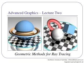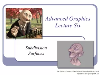
Advanced Graphics Lecture Six
330 likes | 367 Vues
Explore the transition from NURBS patches to subdivision surfaces for improved continuity and practicality in computer graphics. Learn about historical developments, applications in CAD/CAM and animation, and the significance of schemes like Chaikin, Doo-Sabin, and Catmull-Clark.

Advanced Graphics Lecture Six
E N D
Presentation Transcript
Advanced GraphicsLecture Six Subdivision Surfaces Alex Benton, University of Cambridge – A.Benton@damtp.cam.ac.uk Supported in part by Google UK, Ltd
NURBS patches • NURBS patches are (n+1)x(m+1), forming a mesh of quadrilaterals. • What if you wanted triangles or pentagons? • A NURBS dodecahedron? • What if you wanted vertices of valence other than four? • NURBS expressions for triangular patches, and more, do exist; but they’re cumbersome.
Problems with NURBS patches • Joining NURBS patches with Cn continuity across an edge is annoying. • What happens to continuity at corners where the number of patches meeting isn’t exactly four? • Animation is tricky: bending and blending are doable, but not easy. Sadly, the world is not made up of shapes that can be made from one smoothly-deformed rectangular surface.
Subdivision surfaces • Beyond shipbuilding: we want guaranteed continuity, without having to build everything out of rectangular patches. • Applications include CAD/CAM, 3D printing, museums and scanning, medicine, movies… • The solution: subdivision surfaces. Geri’s Game, by Pixar (1997)
Subdivision surfaces • Instead of ticking a parameter t along a parametric curve (or the parameters u,v over a parametric grid), subdivision surfaces repeatedly refine from a coarse set of control points. • Each step of refinement adds new faces and vertices. • The process converges to a smooth limit surface. (Catmull-Clark in action)
Subdivision surfaces – History • de Rahm described a 2D (curve) subdivision scheme in 1947; rediscovered in 1974 by Chaikin • Concept extended to 3D (surface) schemes by two separate groups during 1978: • Doo and Sabin found a biquadratic surface • Catmull and Clark found a bicubic surface • Subsequent work in the 1980s (Loop, 1987; Dyn [Butterfly subdivision], 1990) led to tools suitable for CAD/CAM and animation
Subdivision surfaces and the movies • Pixar first demonstrated subdivision surfaces in 1997 with Geri’s Game. • Up until then they’d done everything in NURBS (Toy Story, A Bug’s Life.) • From 1999 onwards everything they did was with subdivision surfaces (Toy Story 2, Monsters Inc, Finding Nemo...) • It’s not clear what Dreamworks uses, but they have recent patents on subdivision techniques.
Useful terms • A scheme which describes a 1D curve (even if that curve is travelling in 3D space, or higher) is called univariate, referring to the fact that the limit curve can be approximated by a polynomial in one variable (t). • A scheme which describes a 2D surface is called bivariate, the limit surface can be approximated by a u,v parameterization. • A scheme which retains and passes through its original control points is called an interpolating scheme. • A scheme which moves away from its original control points, converging to a limit curve or surface nearby, is called an approximating scheme. Control surface for Geri’s head
How it works • Example: Chaikin curve subdivision (2D) • On each edge, insert new control points at ¼ and ¾ between old vertices; delete the old points • The limit curve is C1 everywhere (despite the poor figure.)
Even • Odd Notation • Chaikin can be written programmatically as: • …where k is the ‘generation’; each generation will have twice as many control points as before. • Notice the different treatment of generating odd and even control points. • Borders (terminal points) are a special case.
Notation • Chaikin can be written in vector notation as:
Notation • The standard notation compresses the scheme to a kernel: • h =(1/4)[…,0,0,1,3,3,1,0,0,…] • The kernel interlaces the odd and even rules. • It also makes matrix analysis possible: eigenanalysis of the matrix form can be used to prove the continuity of the subdivision limit surface. • The details of analysis are fascinating and beyond the scope of this course; check out Malcolm Sabin’s lecture series, “Computer Aided Geometric Design”, over at the CMS. • The limit curve of Chaikin is a quadratic B-spline!
Reading the kernel • Consider the kernel • h=(1/8)[…,0,0,1,4,6,4,1,0,0,…] • You would read this as • The limit curve is provably C2-continuous.
Making the jump to 3D: Doo-Sabin • Doo-Sabin takes Chaikin to 3D: • P = (9/16)A + (3/16)B + (3/16)C + (1/16)D • This replaces every old vertex with four new vertices. • The limit surface is biquadratic, C1 continuous everywhere. D C P B A
Doo-Sabin in action (0) 18 faces (1) 54 faces (2) 190 faces (3) 702 faces
Catmull-Clark • Catmull-Clark is a bivariate approximating scheme with kernel h=(1/8)[1,4,6,4,1]. • Limit surface is bicubic, C2-continuous. 6 4 4 1 1 Vertex 16 16 24 24 6 6 Face 36 16 16 4 4 1 1 Edge 6 /64
Vertex rule Face rule Edge rule Catmull-Clark • Getting tensor again:
Catmull-Clark vs Doo-Sabin Doo-Sabin Catmull-Clark
Extraordinary vertices • Catmull-Clark and Doo-Sabin both operate on quadrilateral meshes. • All faces have four boundary edges • All vertices have four incident edges • What happens when the mesh contains extraordinary vertices or faces? • Extraordinary vertex: not the assumed degree. • For many schemes, adaptive weights exist which can continue to guarantee at least some (non-zero) degree of continuity, but not always the best possible. • CC replaces extraordinary faces with extraordinary vertices; DS replaces extraordinary vertices with extraordinary faces. Detail of Doo-Sabin at cube corner
Extraordinary vertices: Catmull-Clark • Catmull-Clark vertex rules generalized for extraordinary vertices: • Original vertex: • (4n-7) / 4n • Immediate neighbors in the one-ring: • 3/2n2 • Interleved neighbors in the one-ring: • 1/4n2 Image source: “Next-Generation Rendering of Subdivision Surfaces”, Ignacio Castaño, SIGGRAPH 2008
Loop scheme: Butterfly scheme: 1 1 0 0 10 16 1 1 0 0 Split each triangle into four parts 1 1 0 0 0 0 -1 -1 2 6 2 2 8 8 2 6 0 0 -1 -1 Schemes for simplicial (triangular) meshes Vertex Vertex Edge Edge (All weights are /16)
Loop subdivision Loop subdivision in action. The asymmetry is due to the choice of face diagonals.Image by Matt Fisher, http://www.its.caltech.edu/~matthewf/Chatter/Subdivision.html
Creases • Extensions exist for most schemes to support creases, vertices and edges flagged for partial or hybrid subdivision.
Continuous level of detail • For live applications (e.g. games) can compute continuous level of detail, e.g. as a function of distance: Level 5.2 Level 5.8 Level 5
Direct evaluation of the limit surface • In the 1999 paper Exact Evaluation Of Catmull-Clark Subdivision Surfaces at Arbitrary Parameter Values,Jos Stam (now at Alias|wavefront) describes a method for finding the exact final positions of the CC limit surface. • His method is based on calculating the tangent and normal vectors to the limit surface and then shifting the control points out to their final positions. • What’s particularly clever is that he gives exact evaluation at the extraordinary vertices. (Non-trivial.)
Bounding boxes and convex hulls for subdivision surfaces • The limit surface is the weighted average of the weighted averages of [repeat for eternity…] the original control points. • This implies that for any scheme where all weights are positive and sum to one, the limit surface lies entirely within the convex hull of the original control points. • For schemes with negative weights: • Let L=maxt Σi |Ni(t)| be the greatest sum throughout parameter space of the absolute values of the weights. • For a scheme with negative weights, L will exceed 1. • Then the limit surface must lie within the convex hull of the original control points, expanded unilaterally by a ratio of (L-1).
Splitting a subdivision surface • Many iterrogations rely on subdividing and examining the bounding boxes of the smaller facets. • Or just chop the geometry in half! • Find new bounding boxes: not just the bounding boxes of the control points of the new geometry • Need to include all control points from the previous generation, which influence the limit surface in this smaller part. • That’ll extend further, beyond the local control points. • Need to extend to include all local support. (Top) 5x Catmull-Clark subdivision of a cube (Bottom) 5x Catmull-Clark subdivision of two halves of a cube; the limit surfaces are clearly different.
Ray/surface intersection • To intersect a ray with a subdivision surface, we recursively split and split again, discarding all portions of the surface whose bounding boxes / convex hulls do not lie on the line of the ray. • Any subsection of the surface which is ‘close enough’ to flat is treated as planar and the ray/plane intersection test is used. • This is essentially a binary tree search for the nearest point of intersection. • You can optimize by sorting your list of subsurfaces in increasing order of distance from the origin of the ray.
Rendering subdivision surfaces • The algorithm to render any subdivision surface is exactly the same as for Bezier curves: • “If the surface is simple enough, render it directly; otherwise split it and recurse.” • One fast test for “simple enough” is, • “Is the convex hull of the limit surface sufficiently close to flat?” • Caveat: splitting a surface and subdividing one half but not the other can lead to tears where the different resolutions meet. →
Rendering subdivision surfaces on the GPU • Recent work (2005) has shown how to render subdivision surfaces in hardware using the GPU. • This subdivision can be done completely independently of geometry, imposing no demands on the CPU. • Uses a complex blend of precalculated weights and shader logic • Impressive effectsin use at id, Valve,etc! Figure from Generic Mesh Renement on GPU, Tamy Boubekeur & Christophe Schlick (2005) LaBRI INRIA CNRS University of Bordeaux, France
Approximating Quadrilateral (1/2)[1,2,1] (1/4)[1,3,3,1] (Doo-Sabin) (1/8)[1,4,6,4,1] (Catmull-Clark) Mid-Edge Triangles Loop Interpolating Quadrilateral Kobbelt Triangle Butterfly “√3” Subdivision Many more exist, some much more complex This is a major topic of ongoing research Subdivision Schemes—Summary
References • Catmull, E., and J. Clark. “Recursively Generated B-Spline Surfaces on Arbitrary Topological Meshes.” Computer Aided Design, 1978. • Dyn, N., J. A. Gregory, and D. A. Levin. “Butterfly Subdivision Scheme for Surface Interpolation with Tension Control.” ACM Transactions on Graphics. Vol. 9, No. 2 (April 1990): pp. 160–169. • Halstead, M., M. Kass, and T. DeRose. “Efficient, Fair Interpolation Using Catmull-Clark Surfaces.” Siggraph ‘93. p. 35. • Zorin, D. “Stationary Subdivision and Multiresolution Surface Representations.” Ph.D. diss., California Institute of Technology, 1997 • Ignacio Castano, “Next-Generation Rendering of Subdivision Surfaces.” Siggraph ’08, http://developer.nvidia.com/object/siggraph-2008-Subdiv.html • Dennis Zorin’s SIGGRAPH course, “Subdivision for Modeling and Animation”, http://www.mrl.nyu.edu/publications/subdiv-course2000/