Download
1 / 34
340 likes | 363 Vues
Explore sound modal analysis, harmonic motion, spring-mass systems, and fluid-structure interaction. Learn the dynamics of vibrating objects and how to simulate their responses.

E N D
COMP768-F16 Course Presentation Sound Modal Analysis, Synthesis, and Fluid-Structure Interaction Justin Wilson
Labeling Conventions • Upper case denotes matrix and lower case denotes vector or scalar • May see damping noted as C or D • Damping labeled as D or d in this presentation • May see displacement (current position – resting position) as x, r, or u • 3D displacement labeled as u • 1D displacement labeled as x • Rayleigh damping coefficients as η and δ, α and β, or α1 and α2 • Rayleigh damping coefficients labeled as α1 and α2 in this presentation • May see mode space matrix as Φ or U • Mode space matrix labeled as U in this presentation • May see displacement in mode space as z or q • Displacement in mode space labeled as q in this presentation • Fluid-Structure Interaction (aka Elasto-Acoustics, aka Solid-Fluid Interface)
Discussion topics • Sound modal analysis • How do we hear sound? • What properties influence the sound of an object? • How can we perform sound modal analysis? • Sound modal synthesis • Fluid-Structure Interaction • What causes an object to make a sound when it is struck?
Sound waves and harmonic motion • When an object is struck, it vibrates and deforms • The surrounding air rapidly compresses (compression) and expands (rarefaction or decompression) as the object vibrates outward and inward respectively • As it oscillates periodically, pressure waves are created and air pressure amplitude changes up and down in over time (like a sine wave) • Although we may not see the vibrations or deformations, our ears hear the variation in air pressure as sound • Harmonic motion (aka harmonic oscillation) is the periodic pattern of compression and rarefaction Pressure waves Source: digitalsoundandmusic.com
A spring-mass system is also a vibration model • Like harmonic motion, a spring mass system also responds in a periodic motion • Undamped case (d=0) • mx’’(t) + kx(t) = 0 • Amplitude does not decrease with time • Damped case (d > 0) • mx’’(t) + dx’(t) + kx(t) = 0 • Underdamped case (0 < d2 < 4*k*m) • Amplitude vibrates but eventually stops • ω = • Critically damped case (d = 4*k*m) • Decays to zero without oscillating • Overdamped case (d > 4*k*m) • Also decays to zero without oscillating Undamped case Source: digitalsoundandmusic.com Underdamped case
Sound dynamics equation • Mu’’ + Du’ + Ku = f • M = mass matrix, where mass is located on the object • u = vector of the displacement of each element • vector of all zeros represent object at rest • n elements for object, then u vector size = 3n (x,y,z position) • D = viscous damping matrix, how velocity decays over time • K = stiffness matrix, defines connectivity of the elements • f = vector of forces, inducing vibrations • Given these parameters, we can simulate the vibration of the solid volume bodyobject in response to an impulse • Then, how do we represent the object anddetermine its parameter values (M, D, K)? Source: SIGGRAPH 2016 Course Notes
Rigid body sound pipeline • Generate volumetric mesh • Construct the stiffness K, mass M, & damping D matrices • Run generalized eigen-decomposition • Construct the decoupled modal vibration equations • Numerically integrate individual modes
Object is a volumetric solid body Single tetrahedron of finite element mesh • Represent surface mesh with a finite element mesh (e.g. tetrahedral) • Tetrahedral mesh has n nodes where i=1…n • Xi are the rest positions • xi(t) is the time-varying displaced position • ui(t) = (xi(t) – Xi) is the nodal displacement • Mu’’ + Du’ + Ku = f(t) • High-dimensional equivalent to spring-mass mx’’(t) + dx’(t) + kx(t) = f(t) • M, D, and K are size 3n x 3n sparse matrices u1x u1y u1z u2x … 3n x 1 vector of displacement vectors ui of all nodes u = = ui Pressure waves xi Source: digitalsoundandmusic.com Xi
Rigid body sound pipeline • Generate volumetric mesh • Construct the stiffness K, mass M, & damping D matrices • Run generalized eigen-decomposition • Construct the decoupled modal vibration equations • Numerically integrate individual modes
Stiffness matrix K (parameters) Single tetrahedron of finite element mesh • Stiffness describes element connectivity • If the tetrahedra are small, then can approximate: • Deformation gradient as a constant value inside of each tetrahedron • F = [x2 – x1 x3 – x1 x4 – x1][X2 – X1 X3 – X1 X4 – X1] -1 • Strain also as a constant and linearized since the vibration is very tiny • E = ½ * (F + FT) • Stress tensor S = -C*E (linear constitutive law, aka Hooke’s law) • Strain tensor E and stiffness tensor C (symmetric 4th order tensor) • Stiffness tensor C depends on the material; for isotropic materials: • Cijkl = Kδijδkl + µ(δikδjl + δilδjk − 2/3*δijδkl) where δij is the Kronecker delta function • Given a stress tensor S & direction n, elastic force is Sn • n1 = effective normal of node 1 = average of three adjacent triangle normals Source: SIGGRAPH 2016 Course Notes
Stiffness matrix K (related to force) Single tetrahedron of finite element mesh • Total internal force at node j = fj = ∑ Sinji(summed over i ∈ Tj) • Tj indicates set of tetrahedral that include node j • nji is the effective normal n of node j for tetrahedron i • Si is the constant stiffness tensor S for tetrahedron i • Since njiis a constant direction and Si is linearly related to nodal positions xi, we can express f = Ku (similar to mass-spring kx(t)) • Rewrite Si which is linearly related to nodal position xi with K which is a linear function with respect to the displacement vectors uj • Strain state in a solid medium around some point cannot be described by a single vector • f stacks internal force vectors of all finite element nodes • K is a sparse matrix because each node depends only on surrounding tetrahedra Source: SIGGRAPH 2016 Course Notes
Stiffness matrix key takeaways • Based on elements of the object’s volumetric mesh & Poisson’s ratio • Poisson’s ratio for most materials range between 0 (cork) and 0.5 (rubber), typically between 0.15 and 0.35 • When a material is compressed in one direction, it usually tends to expand in the other two directions • Poisson’s ratio ν = (% expansion) / (% compression) • stiffness_ssh “solver” based on UNC (Huai-Ping) • Inputs • .ele and .node files generated from Tetgen • Poisson’s ratio • Ouput • Stiffness matrix elements Poisson’s ratio for different materials
Mass matrix key takeaways • Mass matrix construction methods • Direct Mass Lumping (DML) • Variational Mass Lumping (VML) • Consistent Mass Matrix (CMM) • Template Mass Lumping (TML) • Compute mass matrix using "volumetricMesh“ library [Barbic] • This library uses consistent mass matrix (CMM) of a tetrahedron • Eigenvectors are mass-normalized
Damping matrix D (Rayleigh damping) • Rayleigh damping (aka linearly proportional damping) is used to model losses based on mass and stiffness • Rayleigh damping: D = α1M + α2K • Linear combination of mass (M) and stiffness (K) where α1 and α2 are real-valued parameters • Rayleigh damping is most commonly used because of ease of computation but note the following limitations: • Rayleigh damping is only a first-order approximation • Originally chosen for ease of computation, not its physical accuracy • Only produces normal modes • Other damping models • Caughey damping • Generalized proportional damping (GPD)
Mass, stiffness, and damping “solvers” • Mass (M) and stiffness (K) can be constructed through knowledge of the shape and material properties of the object • Notably, its density (p), Poisson’s ratio (ν), and Young’s modulus (E) • Damping (D), how do we obtain the Rayleigh coefficients α1 and α2? • Instead of by hand, researchers1 have established a method to automatically estimate them from recorded audio • Glass for example • ν = .25, E = 50e09 Pascals, p = 2500 kg/m3 • α1 = 2.0and α2 = 7.8e-8 1 Example-Guided Physically Based Modal Sound Synthesis [Ren et al]
Rigid body sound pipeline • Generate volumetric mesh • Construct the stiffness K, mass M, & damping D matrices • Run generalized eigen-decomposition • Construct the decoupled modal vibration equations • Numerically integrate individual modes
Eigendecomposition • Shape and material properties of the object are analyzed to decompose the vibrations into a set of modes of vibration • Linear combination of normal modes with different amplitudes, frequencies, and phases • We perform generalized eigenvalue decomposition using KU = MUS and displacement vector u = Uq • U is the modal shape matrix of normal modes, containing the eigenvectors • S is the diagonal eigenvalue matrix • Mu’’ + Du’ + Ku = f(t), set u = Uq, and multiply by UT • UTMUq’’ + UTDUq’ + UTKUq = UTf(t) • Simplify by substituting UTMU = I, UTDU = α1I + α2S, and UTKU = S • q’’ + (α1I + α2S)q’ + Sq = UTf(t) • General eigendecomposition solver using Intel MKL (Math Kernel Library) to obtain eigenvalues
Rigid body sound pipeline • Generate volumetric mesh • Construct the stiffness K, mass M, & damping D matrices • Run generalized eigen-decomposition • Construct the decoupled modal vibration equations • Numerically integrate individual modes
Rather than solving a set of coupled equations, wesolve n damped vibration independent equations • Matrices UTMU = I, UTDU = α1I + α2S, and UTKU = S are diagonal so equations about q are independent • So can solve n damped vibration equations independently • We decouple Mu’’ + Du’ + Ku = f(t) into a set of independent 1D vibration equations mx’’(t) + dx’(t) + kx(t) = 0 • q’’ + (α1I + α2S)q’ + Sq = UTf(t) • Damping di = α1+ α2 * eigenvaluei • Stiffness ki = eigenvaluei • UTf(t) is the force vector represented with mode coordinates • Remember, ωi = 2πfi and mass matrix is mass normalized so m = 1 • For the purpose of sound synthesis, we are interested in the vibrational frequencies in our hearing range (20Hz to 20kHz) • Therefore, we only need to consider modes with vibrational frequencies in this range ω = frequency f = π
Rigid body sound pipeline • Generate volumetric mesh • Construct the stiffness K, mass M, & damping D matrices • Run generalized eigen-decomposition • Construct the decoupled modal vibration equations • Numerically integrate individual modes
Numeric methods • In general, each natural mode of the system has a different natural frequency • The physical interpretation of the eigenvalues and eigenvectors which come from solving the system are that they represent the frequencies and corresponding mode shapes • Harmonic Oscillator [Barbic] • Integrates a single 1D harmonic oscillator; can timestep the following Ordinary Differential Equation: M * q''(t) + D * q'(t) + K * q(t) = f(t) • Only supports underdamped systems • Modal superposition analysis (aka modal analysis) • Modal expansion thereom Source: MIT Open Courseware [Vandiver]
Summary of modal analysis steps • Analyze the vibrations of the sounding object (Mu’’ + Du’ + Ku = f(t)) • Parameters based on shape and material set of properties • Stiffness matrix • Mass matrix • Using tetrahedral nodes, Poisson’s ratio, Young’s modulus, and density • Damping model: how vibrations of a modeled object will decay over time • Rayleigh damping (aka linearly proportional damping of mass and stiffness) • Mode space (q’’ + (α1I + α2S)q’ + Sq = Utf(t)) • Damping di = α1+ α2 * eigenvaluei • Stiffness ki = eigenvaluei • UTf(t) converts forces on elements to normal mode amplitudes • Frequency fi • Dynamically create sounds at runtime with modal synthesis = π
Modal sound synthesis • Simulate based on a contact point • Position (x,y,z) of where the object is struck • ANN (Approximate Nearest Neighbor) [Mount and Arya] • Impulse direction (x,y,z); e.g. usually striking the object in normal direction to the contact point but could synthesize tangentially to the object like (0,1,0) • Synthesis Toolkit in C++ (STK) [Cook and Scavone] • C++ open source audio signal processing and algorithmic synthesis • Realtime audio in C++ (RtAudio) [Scavone] • RtAudio provides a common API for realtime audio input/output
Real-time sound synthesis • To achieve real-time, these pre-processing steps are performed for a given object and material • Eigendecomposition is performed and resulting UT and each mode’s damping coefficient d and damped frequency fiare saved • At run-time, an applied force f is transformed to mode space UTf • Resulting q vector from UTf contains the amplitudes with which to scale each mode • Sampled sound equals some of the mode amplitudes • Resulting damped sinusoids q(t) can be combined and sampled at 44kHz to produce the sound • Based on Nyquist theorem should sample at double what humans can sense • For example, if we choose a samping rate of 48kHz, then deltaT = 1.0 / 48kHz ~ 0.00002 Example-Guided Physically Based Modal Sound Synthesis [Ren et al]
Fluid-Structure Interaction and Elasto-Acoustic coupling • Elasto-acoustic coupling may also be referred to as solid-fluid interface • It involves the interactions between the vibrations of an elastic structure and the sound field in the surrounding fluid • Weak coupling may be used if the pressure forces of the fluid on the solid are negligible, then a sequential computation can be formed • Mechanical surface vibrations are calculated first and then used as the input for an acoustic field computation • Strong coupling requires that the mechanical and acoustic field equations including couplings be solved simultaneously
FSI overview diagram Τs • Two independently Τs and Τf generated triangulations on Ωs and Ωf • Displacement u on Τs • Potential ψ on Tf • Two (d−1)-dimensional grids ∂Τs and ∂Tf on interface boundary ΓI • At the interface ΓI we have to consider the solid - fluid coupling • n ⋅ (vs – vf) = 0 = n ⋅ u’ + ∂ψ/∂n • [σ] ⋅ n + pfnψ’ = 0 Τf ΓI Elasto-Acoustic and Acoustic-Acoustic Coupling on Nonmatching Grids [Flemisch et. al]
Displacement vs. potential-based formulation • So we can use standard Lagrangian nodal finite elements in both domains, we use: • Displacement-based formulation for the solid (u) • Potential-based formulation for the fluid (ψ) • If both solid and fluid used displacement-based formulations, then would require non-standard discretization by means of Raviart-Thomas
Discretized elasto-coupling dynamics equation • Block diagonal entries Mu, Mψ, Dψ, Ku, Kψcan be assembled locally without needing any information from the opposite grid • Coupling between the two grids takes place Duψ and DTuψ which realize the boundary integrals • Duψ = [Dpq] = ∈ Rd • Terms defined on next slide Mu 0 0 -Mψ u’’ ψ’’ 0 Duψ DTuψ -Dψ u’ ψ’ Ku 0 0 -Kψ u ψ fu 0 + + =
Algorithm • Duψ = [Dpq] = ∈ Rd • is scalar basis functions associated with node p on dΤs • is scalar basis functions associated with node q on dΤf • pf is the mean density of the fluid • Γ is the boundary between fluid-structure interface • Τs and Τfare surface and fluid triangulations respectively • n is the normal at the boundary point • The key to this equation/algorithm is the determination of the intersection area of two elements from the different grids • Intersection determined if a vertex lies inside the other surface element en or vice versa • For 3D, complexity order O(n4/3) with n denoting total # of unknowns • It is possible to do better by incorporating neighbor relations of the surface elements and/or inheritance relations from an underlying geometrical multigrid hierarchy
Algorithm (continued) • for all slave elements eni, i = 1, …, nn do • for all master elements emj, j = 1, …, nm do • determine intersection are enm = eni∩ emj • if eij != 0 then • for all basis function Nm, ɸn with support ∩ eij!= 0 do • add ∫enmNmɸn dΓ to M • end for • end if • end for • end for Elasto-Acoustic and Acoustic-Acoustic Coupling on Nonmatching Grids [Flemisch et. al]
Research References • Physically Based Sound for Computer Animation and Virtual Environments [ACM SIGGRAPH 2016 Course] • Modal Vibration • Acoustic Transfer • Example-Guided Physically Based Modal Sound Synthesis [Ren et al] • Interactive Modal Sound Synthesis Using Generalized Proportional Damping [Sterling et al] • Elasto-Acoustic and Acoustic-Acoustic Coupling on Nonmatching Grids [Flemisch et. al] • Q. Elasto-Acoustics in Formulas of Acoustics [Maysenholder and Mechel] • Fluid-Structure Interaction: Applied Numerical Methods [Morand and Ohayon]
Software Libraries • Volumetric Mesh library [Barbic] • Tetgen to volumetric mesh • Computes mass matrix • Intel MKL (Math Kernel Library) • General eigendecomposition • Synthesis Toolkit in C++ (STK) [Cook and Scavone] • Set of open source audio signal processing and algorithmic synthesis C++ classes • Harmonic Oscillator [Barbic] • Integrates a single 1D harmonic oscillator; can timestep the following Ordinary Differential Equation: M * q''(t) + D * q'(t) + K * q(t) = f(t) • ANN (Approximate Nearest Neighbor) [Mount and Arya] • Supports exact and approximate nearest neighbor searching in arbitrarily high dimensions
Thank You and Happy Halloween! • Questions?