Association analysis
Association analysis. Genetics for Computer Scientists 15.3.-19.3.2004 Biomedicum & Department of Computer Science, Helsinki Päivi Onkamo. Lecture outline. Genetic association analysis Allelic association χ 2 –test Linkage disequilibrium (LD) process

Association analysis
E N D
Presentation Transcript
Association analysis Genetics for Computer Scientists 15.3.-19.3.2004 Biomedicum & Department of Computer Science, Helsinki Päivi Onkamo
Lecture outline • Genetic association analysis • Allelic association • χ2 –test • Linkage disequilibrium (LD) process • Formulation of the computational problem for LD mapping • Limitations of the LD mapping • Approaches. For example: HPM
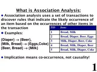
Genetic association analysis • Search for significant correlations between gene variants and phenotype • For example: Locus A for SLE: 100 cases and 100 controls genotyped
Allelic association = An allele is associated to a trait • Allele 1 seems to be associated, based on sheer numbers, but how sure can one be about it?
Affected Healthy Allele 1 79 46 125 Allele 2 21 54 75 100 100 200
The idea is to compare the observed frequencies to frequencies expected under hypothesis of no association between alleles and the occurrence of the disease (independency between variables) • Test statistic Where • oi is the observed class frequency for class i, ei expected (under H0 of no association) • k is the number of classes in the table • Degrees of freedom for the test: df=(r-1)(s-1)
Affected Healthy Allele 1 62.5 (79) 62.5 (46) 125 Allele 2 37.5 (21) 37.5 (54) 75 100 100 200 Expected df=1 p<<0,001
Interpretation of the test results • The p-value is low enough that H0 can be rejected = the probability that the observed frequencies would differ this much (or even more) from expected by just coincidence < 0.001 • χ2 –tables (Appendix), internet resources, etc.
Genetic association is population levelcorrelation with some known genetic variant and a trait: an allele is over-represented in affected individuals → • From a genetic point of view, an association does not imply causal relationship • Often, a gene is not a direct cause for the disease, but is in LD with a causative gene →
Linkage disequilibrium (LD) • Closely located genes often express linkage disequilibrium to each other: Locus 1 with alleles A and a, and locus 2 with alleles B and b, at a distance of a few centiMorgans from each other • At equilibrium, the frequency of the AB haplotype should equal to the product of the allele frequencies of A and B, AB = AB. If this holds, then Ab = A b, aB = aB and ab = ab , as well. Any deviation from these valuesimplies LD.
Linkage disequilibrium (LD) • LD follows from the fact that closely located genes are transmitted as a ”block” which only rarely breaks up in meioses • An example: • Locus 1 – marker gene • Locus 2 – disease locus, with allele b as dominant susceptibility allele with 100% penetrance
Association evaluated → Locus 1 also seems associated, even though it has nothing to do with the disease – association observed just due to LD LD mapping – utilizing founder effect • A new disease mutation born n generations ago in a relatively small, isolated population • The original ancestral haplotype slowly decays as a function of generations • In the last generation, only small stretches of founder haplotype can be observed in the disease-associated chromosomes
Data: Searching for a needle in a haystack Disease gene Disease status SNP1 S2 ... ... a ? 2 1 1 a ? 1 2 1 1 2 2 1 1 2 1 2 1 2 1 1 2 2 1 2 2 1 2 1 1 2 2 1 1 1 1 1 1 1 c 2 1 ? ?c 1 1 ? ? 1 2 2 1 1 2 1 1 2 2 2 1 1 1 a 1 1 2 1a 1 1 1 2 1 1 2 1 1 2 2 2 2 2 1 1 2 1 2 2 ? 1 1 1 ? 1 … … … …
Task is to find either an allele or an allele string (haplotype) which is overrepresented in disease-associated chromosomes • markers may vary: SNPs, microsatellites • populations vary: the strength of marker-to-marker LD • Many approaches: • ”old-fashioned” allele association with some simple test (problem: multiple testing) • TDT; modelling of LD process: Bayesian, EM algorithm, integrated linkage & LD
Limitations of the LD mapping • The relationship between the distance of the markers vs. the strength of LD: theoretical curve
Linkage disequilibrium (D’) for the African American (red) and European (blue) populations binned in 5 kb classes after removing all SNPs with minor allele frequencies less than 20%. 3429 SNPs were included (Source http://www.fhcrc.org/labs/kruglyak/PGA/pga.html)
Limitations: LD is random process • LD is a continuous process, which is created and decreased by several factors: • genetic drift • population structure • natural selection • new mutations • founder effect → limits the accuracy of association mapping
Research challenges … • Haplotyping methods needed as prerequisite for association/LD methods • …or, searching association directly from genotype data (without the haplotyping stage) • Better methods for measurement of the association (and/or the effects of the genes) • Taking disease models into consideration
A methodological project:Haplotype Pattern Mining (HPM)AJHG 67:133-145, 2000 • Search the haplotype data for recurrent patterns with no pre-specified sequence • Patterns may contain gaps, taking into consideration missing and erroneous data • The patterns are evaluated for their strength of association • Markerwise ‘score’ of association is calculated
Algorithm • Find a set of associated haplotype patterns • number of gaps allowed (2) • maximum gap length (1 marker) • maximum pattern length (7 markers) • association threshold (2 = 9) • Score loci based on the patterns • Evaluate significance by permutation tests • Extendable to quantitative traits • Extendable to multiple genes
Example: a set of associated patterns Marker 01 02 03 04 05 06 07 08 2 P1 2 1 2 2 2 * * * 9.6 P2 2 1 2 2 2 1 * * 9.2 P3 2 1 2 2 * 1 1 * 8.9 P4 2 1 * 2 1 * * * 8.1 P5 1 * 1 2 2 * * * 7.4 P6 * * 1 2 2 1 2 * 7.1 P7 * 2 1 2 * * * * 7.1 P8 2 1 1 2 * * * * 6.9 P9 2 1 1 * * * * * 6.8 Score 5 6 7 7 6 3 2 0
Pattern selection • The set of potential patterns is large. • Depth-first search for all potential patterns • Search parameters limit search space: • number of gaps • maximum gap length • maximum pattern length • association threshold
Permutation tests • random permutation of the status fields of the chromosomes • 10,000 permutations • HPM and marker scores recalculated for each permuted data set • proportion of permuted data sets in which score > true score empirical p-value.
Permutation surface (A=7.5 %). The solid line is the observed frequency.
Localization power with simulated SNP data (density 3 SNPs per 1 cM). Isolated population with a 500-year history was simulated. Disease model was monogenic with disease allele frequency varying from 2.5-10 % in the affecteds. 12.5 % of data was missing. Sample size 100 cases and 100 controls.
Benefits & drawbacks • Non-parametric, yet efficient approach; no disease model specification is needed + • Powerful even with weak genetic effects and small data sets + • Robust to genotyping errors, mutations, missing data + • Allows for gaps in haplotypes +
Flexible: easily extended to different types of markers, environmental covariates, and quantitative measurements + • optimal pattern search parameters may need to be specified case-wise - • no rigid statistical theory background - • requires dense enough map to find the area where DS gene is in LD with nearby markers.
Search of the susceptibility gene: • With good luck - and information from gene banks, pick up the correct candidate gene • Genetic region with positive linkage signal is saturated with markers, and this data is now searched for a secondary correlation – correlation of marker allele(s) with the actual disease mutation (LD)
Improved statistical methods to detect LD • Terwilliger (1995) • Devlin, Risch, Roeder (1996) • McPeek and Strahs (1999) • Service, Lang et al. (1999) • Statistical power of association test statistics • Long, Langley (1999). • Review on statistical approaches to gene mapping • Ott, Hoh (2000)