Association Analysis (7) (Mining Graphs)
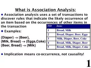
Association Analysis (7) (Mining Graphs). Frequent Subgraph Mining. Extend association rule mining to finding frequent subgraphs Useful for Web Mining, computational chemistry, spatial data sets, etc. Homepage. Teaching. Databases. Data Mining. Bio/Chem-Informatics.

Association Analysis (7) (Mining Graphs)
E N D
Presentation Transcript
Frequent Subgraph Mining • Extend association rule mining to finding frequent subgraphs • Useful for Web Mining, computational chemistry, spatial data sets, etc Homepage Teaching Databases Data Mining
Bio/Chem-Informatics • Each year, new chemical compounds are designed. • We know that structure of a compound plays a big role in its chemical properties. • However, it is difficult to establish their exact relationship. • Frequent subgraph mining can aid by identifying the substructures commonly associated with certain properties of known compounds.
Widom Calvanese Jeff Ullman Vardi Garcia-Molina Lenzerini Alfred Aho Kuperferman A mined subgraph Web mining • E.g. Mining the DBLP Web Graph Two examples of matches
Apriori-Like Approach • Support: • number of graphs that contain a particular subgraph • Apriori principle still holds • Level-wise (Apriori-like) approach: • Vertex growing: • k is the number of vertices • Edge growing: • k is the number of edges
Apriori-Like Algorithm • Generate candidate • Merge pairs of frequent (k - 1)-subgraphs to obtain a candidate k-subgraphs. • Prune candidates • Discard all candidate k-subgraphs that contain infrequent (k - l)-subgraphs. • Count support • Counting the number of graphs in DBthat contain each candidate. • Discard all candidate subgraphs whose support counts are less than minsup.
Vertex Growing r The resulting matrix is the first matrix, appended with the last row and last column of the second matrix. The remaining entries of the new matrix are either zero or replaced by all valid edge labels connecting the pair of vertices.
Edge Growing Edge growing inserts a new edge to an existing frequent subgraph during candidate generation. Doesn’t necessarily increase the number of vertices in the original graphs.
Topological equivalence • Two vertexes are topologically equivalent if they have: • The same label and • The same number and label of edges incident to them. v1,v4 are topologically equivalent v2,v3 are topologically equivalent No topologically equivalent vertexes v1,v2,v3,v4 are topologically equivalent
v v1 p v2 a a a e p q q q + r r r d e d b b b q q p p p c c c v’ Multiplicity of Candidates Case 1a: vv’ , v1v2 (Topologically in the (k-2)-graphs) Core: The (k-2)-edge subgraph that is common between the joint graphs We try to map the cores.
a p q v r e v1 b a a q v2 p p c q q + r r e e p b b a e q p p c q c r e b v’ q p c Multiplicity of Candidates Case 1b: vv’, v1=v2 (Topologically in the (k-2)-graphs)
v v’ p v2 a a a e v1 q p q q q q + r r r d e d b b b p p p c c c Multiplicity of Candidates Case 2a: vv’ , v1v2(Topologically in the (k-2)-graphs)
p a e q q v v’ r e b a a v2 p v1 q p c q q + r r e e b b p a p p e c c q q r b p c Multiplicity of Candidates Case 2b: vv’, v1=v2(Topologically in the (k-2)-graphs)
p a e v q r d a a q b p q q q + a r r d e q b b q q a a v’ p a e q q r d b q a Multiplicity of Candidates Case 2c: vv’(Topologically in the (k-2)-graphs) We try to map the cores, and there two ways to do this.
p p a a e e v q q q r r e a a q b b p q q q q + a a r r e e q b b q q a a p p a a e e v’ q q q q r r e b b q q a a Multiplicity of Candidates Case 2d: vv’(Topologically in the (k-2)-graphs) We try to map the cores, and there two ways to do this.
Multiplicity of Candidates More than two topologically equivalent vertexes b a c a a a a a b c a b c + a a a a a a a a a a c a Core: The (k-2) subgraph that is common between the joint graphs a b a
A(1) A(2) A(3) A(4) B(5) B(6) B(7) B(8) A(1) 0 1 1 0 1 0 0 0 A(2) 1 0 0 1 0 1 0 0 A(3) 1 0 0 1 0 0 1 0 A(4) 0 1 1 0 0 0 0 1 B(5) 1 0 0 0 0 1 1 0 B(6) 0 1 0 0 1 0 0 1 B(7) 0 0 1 0 1 0 0 1 B(8) 0 0 0 1 0 1 1 0 A(1) A(2) A(3) A(4) B(5) B(6) B(7) B(8) A(1) 0 1 0 1 0 1 0 0 A(2) 1 0 1 0 0 0 1 0 A(3) 0 1 0 1 1 0 0 0 A(4) 1 0 1 0 0 0 0 1 B(5) 0 0 1 0 0 0 1 1 B(6) 1 0 0 0 0 0 1 1 B(7) 0 1 0 0 1 1 0 0 B(8) 0 0 0 1 1 1 0 0 Adjacency Matrix Representation • The same graph can be represented in many ways
Graph Isomorphism • A graph G1 is isomorphic to another graph G2, if G1 is topologically equivalent to G2 • Test for graph isomorphism is needed: • During candidate generation, to determine whether a candidate can be generated • During candidate pruning, to check whether its (k-1)-subgraphs are frequent • During candidate counting, to check whether a candidate is contained within another graph, we should use more specialized algorithms (possibly using indexes with each frequent (k-1) sub-graph)
A(1) A(2) A(3) A(4) B(5) B(6) B(7) B(8) A(1) 0 1 1 0 1 0 0 0 A(2) 1 0 0 1 0 1 0 0 A(3) 1 0 0 1 0 0 1 0 A(4) 0 1 1 0 0 0 0 1 B(5) 1 0 0 0 0 1 1 0 B(6) 0 1 0 0 1 0 0 1 B(7) 0 0 1 0 1 0 0 1 B(8) 0 0 0 1 0 1 1 0 A(1) A(2) A(3) A(4) B(5) B(6) B(7) B(8) A(1) 0 1 0 1 0 1 0 0 A(2) 1 0 1 0 0 0 1 0 A(3) 0 1 0 1 1 0 0 0 A(4) 1 0 1 0 0 0 0 1 B(5) 0 0 1 0 0 0 1 1 B(6) 1 0 0 0 0 0 1 1 B(7) 0 1 0 0 1 1 0 0 B(8) 0 0 0 1 1 1 0 0 Codes Code =1 10 011 1000 01001 001010 0001011 Code =1011010010100000100110001110
Graph Isomorphism • Use canonical labeling to handle isomorphism • Map each graph into an ordered string representation (known as its code) such that two isomorphic graphs will be mapped to the same canonical encoding • Example: • Choose the string representation with the lowest Lexicographical value • Then, the graph isomorphism problem can be solved by string matching.