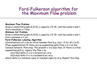
The Ford-Fulkerson Algorithm
The Ford-Fulkerson Algorithm. aka The Labeling Algorithm. Ford-Fulkerson Algorithm. begin x := 0; label node t; while t is labeled do begin unlabel all nodes; pred(j) := 0 for all j in N; label s; LIST := {s}; while LIST is not empty and t is not labeled do


The Ford-Fulkerson Algorithm
E N D
Presentation Transcript
The Ford-Fulkerson Algorithm aka The Labeling Algorithm
Ford-Fulkerson Algorithm begin x := 0; label node t; while t is labeled do begin unlabel all nodes; pred(j) := 0 for all j in N; label s; LIST := {s}; while LIST is not empty and t is not labeled do begin remove a node i from LIST; for all {j in N: (i,j) in A and rij > 0} do if j is unlabeled then pred(j) := i, label j, add j to LIST; end; if t is labeled then augment flow on path from s to t end; end;
(0,2) 2 4 (0,4) (0,5) 1 6 (0,4) t s (0,6) (0,7) (0,5) 3 5 Labeling Algorithm Example
The Residual Network G(x) 2 2 4 4 5 0 1 6 0 0 0 4 t s 6 7 0 5 3 5 0 0
Iteration 1: LIST = {1}, Labeled = {1} i = 1 2 2 4 4 5 0 1 6 0 0 0 4 t s 6 0 7 5 3 5 0 0
Iteration 1: LIST = {1}, Labeled = {1} • i = 1 • LIST = {} • Arc (1,2) • pred(2) =1 • label 2 • LIST = {2} • Arc (1,3) • pred (3) = 1 • label 3 • LIST = {2, 3}
pred(2) = 1 2 2 4 4 5 0 1 6 0 0 0 4 t s 6 7 0 5 3 5 0 0 pred(3) = 1 Iteration 1: LIST = {2,3}, Labeled= {1,2,3}
i = 2 LIST = {3} Arc (2,4) pred(4) =2 label 4 LIST = {3,4} Arc (2,5) pred (5) = 2 label 5 LIST = {3,4,5} Arc (2,1) residual capacity of (2,1) = 0 Iteration 1:LIST = {2,3}, Labeled = {1,2,3}
Iteration 1: LIST = {3,4,5}, Labeled= {1,2,3,4,5} pred(2) = 1 pred(4) = 2 2 2 4 4 5 0 1 6 0 0 0 4 t s 6 7 0 5 3 5 0 0 pred(3) = 1 pred(5) = 2
Iteration 1: LIST = {3,4,5}, Labeled = {1,2,3,4,5} • i = 3 • LIST = {4,5} • Arc (3,5) • 5 is already labeled • Arc (3,1) • residual capacity of (3,1) = 0
Iteration 1: LIST = {4,5}, Labeled = {1,2,3,4,5} • i = 4 • LIST = {5} • Arc (4,2) • residual capacity of (4,2) = 0 • Arc (4,6) • pred(6) =4 • label 6 • LIST = {5,6}
Iteration 1: LIST = {5,6}, Labeled= {1,2,3,4,5,6} pred(2) = 1 pred(4) = 2 2 2 4 4 5 0 pred(6) = 4 1 6 0 0 0 4 t s 6 7 0 5 3 5 0 0 pred(3) = 1 pred(5) = 2
Iteration 1: The sink is labeled • Use pred labels to trace back from the sink to the source to find path P • P = 1 -> 2 -> 4 -> 6 • = min {rij: (i,j) in P) = 2 • Send 2 units of flow from to s to t along path P
(2,2) 2 4 (2,4) (2,5) 1 6 (0,4) t s (0,6) (0,7) (0,5) 3 5 Flow x After Iteration 1 v = 2
The Residual Network G(x) 0 2 4 2 3 2 1 6 2 2 0 4 t s 6 7 0 5 3 5 0 0
Iteration 2: LIST = {1}, Labeled = {1} • i = 1 • LIST = {} • Arc (1,2) • pred(2) =1 • label 2 • LIST = {2} • Arc (1,3) • pred (3) = 1 • label 3 • LIST = {2, 3}
Iteration 2: LIST = {2,3}, Labeled={1,2,3} p=1 0 2 4 2 3 2 1 6 2 2 0 4 t s 6 7 0 5 3 5 0 0 p=1
i = 2 LIST = {3} Arc (2,4) residual cap (2,4) = 0 Arc (2,5) pred (5) = 2 label 5 LIST = {3,5} Arc (2,1) residual capacity of (2,1) = 0 Iteration 2: LIST = {2,3}, Labeled = {1,2,3}
Iteration 2: LIST = {3,5}, Labeled={1,2,3,5} p=1 0 2 4 2 3 2 1 6 2 2 0 4 t s 6 7 0 5 3 5 0 0 p=1 p=2
i = 3 LIST = {5} Arc (3,5) 5 is already labeled Arc (3,1) residual capacity of (3,1) = 0 i = 5 LIST = {} Arc (5,2) residual cap = 0 Arc (5,3) residual cap = 0 Arc (5,6) pred(6) = 5 label 6 LIST = {6} Iteration 2: LIST = {3,5}, Labeled = {1,2,3,5}
Iteration 2: LIST = {6}, Labeled={1,2,3,5,6} p=1 0 2 4 2 3 2 1 6 2 2 0 4 t s 6 7 p=5 0 5 3 5 0 0 p=1 p=2
Iteration 2: The sink is labeled • Use pred labels to trace back from the sink to the source to find path P • P = 1 -> 2 -> 5 -> 6 • = min {rij: (i,j) in P) = 3 • Send 3 units of flow from to s to t along path P
(2,2) 2 4 (2,4) (5,5) 1 6 (3,4) t s (0,6) (3,7) (0,5) 3 5 Flow x After Iteration 2 v = 5
The Residual Network G(x) 0 2 4 2 0 2 1 6 2 5 3 1 t s 6 4 0 5 3 5 0 0
Iteration 3: LIST = {1}, Labeled = {1} • i = 1 • LIST = {} • Arc (1,2) • residual capacity = 0 • Arc (1,3) • pred (3) = 1 • label 3 • LIST = {3}
Iteration 3: List = {3}, Labeled = {1,3} 0 2 4 2 0 2 1 6 2 5 3 1 t s 6 4 0 5 3 5 0 0 p=1
Iteration 3: LIST = {3}, Labeled = {1,3} • i = 3 • LIST = {} • Arc (3,1) • residual capacity = 0 • Arc (3,5) • pred (5) = 3 • label 5 • LIST = {5}
Iteration 3: List = {5}, Labeled = {1,3,5} 0 2 4 2 0 2 1 6 2 5 3 1 t s 6 4 0 5 3 5 0 0 p=1 p=2
Iteration 3: LIST = {5}, Labeled = {1,3,5} • i = 5, LIST = {} • Arc (5,2) • pred(2) = 5 • label 2 • LIST = {2} • Arc (5,3): residual capacity = 0 • Arc (5,6) • pred (6) = 5 • label 6 • LIST = {2,6}
Iteration 3: List = {2,6}, Labeled = {1,2,3,5,6} p=5 0 2 4 2 0 2 1 6 2 5 3 1 t s 6 4 p=5 0 5 3 5 0 0 p=1 p=2
Iteration 3: The sink is labeled • Use pred labels to trace back from the sink to the source to find path P • P = 1 -> 3 -> 5 -> 6 • = min {rij: (i,j) in P) = 4 • Send 4 units of flow from to s to t along path P
(2,2) 2 4 (2,4) (5,5) 1 6 (3,4) t s (4,6) (7,7) (4,5) 3 5 Flow x After Iteration 3 v = 9
The Residual Network G(x) 0 2 4 2 0 2 1 6 2 5 3 1 t s 2 0 7 1 3 5 4 4
Iteration 4: LIST = {1}, Labeled = {1} • i = 1 • LIST = {} • Arc (1,2) • residual capacity = 0 • Arc (1,3) • pred (3) = 1 • label 3 • LIST = {3}
Iteration 4: List = {3}, Labeled = {1,3} 0 2 4 2 0 2 1 6 2 5 3 1 t s 2 0 7 1 3 5 4 4 p=1
Iteration 4: LIST = {3}, Labeled = {1,3} • i = 3 • LIST = {} • Arc (3,1) • 1 is labeled • Arc (3,5) • pred (5) = 3 • label 5 • LIST = {5}
Iteration 4: List = {5}, Labeled = {1,3,5} 0 2 4 2 0 2 1 6 2 5 3 1 t s 2 0 7 1 3 5 4 4 p=3 p=1
Iteration 4: LIST = {5}, Labeled = {1,3,5} • i = 5 • LIST = {} • Arc (5,2) • pred(2) = 5 • label 2 • LIST = {2} • Arc (5,6) • residual capacity = 0
Iteration 4: List = {2}, Labeled = {1,2,3,5} p=5 0 2 4 2 0 2 1 6 2 5 3 1 t s 2 0 7 1 3 5 4 4 p=3 p=1
Iteration 4: LIST = {2}, Labeled = {1,2,3,5} • i = 2 LIST = {} • Arc (2,1) • 1 is already labeled • Arc(2,4) • residual capacity = 0 • Arc (2,5) • 5 is already labeled
Iteration 4: List = {} • The sink is not labeled • Algorithm ends with optimal flow x
Correctness • At the end of each iteration, the algorithm either augments the flow or terminates because it can’t label the sink. • Let S be the set of labeled nodes when the algorithm terminates. Let T = N \ S. • We need to show that when the algorithm terminates v = u[S,T] which implies x is a maximum flow.
Correctness: arcs in (S,T) j s i • rij = 0 • rij = uij - xij + xji • 0 = uij – xij + xji • xij = uij + xji Since xji must be at least zero and 0 xij uij, it follows that xij = uij.
Correctness: arcs in (T,S) s i j • Suppose xij > 0 • rji = uji – xji + xij • Implies rji > 0 (uji xji) • Implies s can reach i in residual network which means i should have been labeled. • Thus, xij = 0
Correctness Thus, the flows on the forward arcs in [S,T] are at the upper bound and there is no flow on any of the backwards arcs. This means x is a maximum flow by Property 6.1.
Complexity • Let U = max {(i,j) in A} uij. • If S = {s} and T = N\{s}, then u[S,T] is at most nU. • The maximum flow is at most nU. • Iteration of the inner while loop is O(m): • Each arc is inspected at most once • Finding is O(n) • Updating the flow on P is O(n) • Complexity is O(nU x m) = O(nmU).