Understanding Image Features in Computer Vision
1.51k likes | 1.64k Vues
This lecture from the University of Texas at Arlington delves into the concept of features in computer vision. Features are any information extracted from images, and the possibilities are infinite. We explore different types of features, including global, region-based, and local features, alongside their utilities in tasks like detection, recognition, and stereo estimation. By examining pixel correspondences and local feature characteristics (like color and small windows), we learn how to find matches between images, which is fundamental for various computer vision applications.

Understanding Image Features in Computer Vision
E N D
Presentation Transcript
Local Features CSE 4310 – Computer Vision Vassilis Athitsos Computer Science and Engineering Department University of Texas at Arlington
What is a Feature? • Any information extracted from an image. • The number of possible features we can define is infinite. • Any function F we can define that takes in an image as an argument and produces one or more numbers as output defines a feature. • Correlation with a template defines a feature. • Projecting to PCA space defines features. • More examples?
What is a Feature? • Any information extracted from an image. • The number of possible features we can define is infinite. • Any function F we can define that takes in an image as an argument and produces one or more numbers as output defines a feature. • Correlation with a template defines a feature. • Projecting to PCA space defines features. • Average intensity. • Std of values in window.
Types of Features • Global features: extracted from the entire image. • Examples: template (the image itself), PCA projection. • Region-based features: extracted from a subwindow of the image. • Any global feature can become a region-based feature by applying it to a specific image region instead of applying it to the entire image. • Local features: describe a pixel, and the vicinity (nearby region) around a specific pixel. • If they describe a “vicinity”, which is a region, one could argue that they are regional features. • The main difference is that a local feature always refers to a specific pixel location. This is not a well-defined or mathematical difference, but it will become clearer when we see examples of local features.
Uses of Features • Features can be used for any computer vision problem. • Detection. • Recognition. • Tracking. • Stereo estimation. • Different types of features work better for different problems, and for different assumptions about the images. • That is why there are many different types of features that people use.
Example: Pixel Correspondences • Are there locations that are visible in both images below? • If so, which pixels correspond to each other? • Even for a human, the answers are not obvious. • Do you see any matching regions? Credit: images downloaded from https://www.cs.ubc.ca/~lowe/keypoints/
Example: Pixel Correspondences • Are there locations that are visible in both images below? • If so, which pixels correspond to each other? • Even for a human, the answers are not obvious. • Do you see any matching regions? Credit: images downloaded from https://www.cs.ubc.ca/~lowe/keypoints/
Example: Pixel Correspondences • Finding correspondences between two images can have different uses. A couple of examples: • 3D estimation using stereo. • Pose estimation: estimating the 3D orientation of an object. • Image stitching: Combining multiple overlapping images into a single image. Credit: images downloaded from https://www.cs.ubc.ca/~lowe/keypoints/
Finding Correspondences • A first approach for finding pixel correspondences: • For each pixel in one image: • Compute the feature vector corresponding to that pixel. • Find the best match for that feature vector in the other image. • If the matching score is better than a threshold, consider it a “match”.
Finding Correspondences • A first approach for finding pixel correspondences: • For each pixel in one image: • Compute the feature vector corresponding to that pixel. • Find the best match for that feature vector in the other image. • If the matching score is better than a threshold, consider it a “match”. • Black boxes that we need to specify: • How do we define feature vectors? We will study several methods. • How do we compute matching scores between two vectors?
Local Feature: Color • The most “local” of all local features is just the color of the pixel. • The feature vector F(i,j) is just the RGB values of the image at pixel (i,j). • Usually, this is not very useful. • Typically, for any pixel in one image, there will be several pixels matching its color in the other image. • This is too “local” to be useful. • A single pixel does not contain much information.
Local Feature: Image Window • We can simply extract a window around the pixel. • We can define a window “half width” h. • Then, given an image G and a pixel location (i,j): Pixel (i,j) Half width: h
Local Feature: Image Window • We can simply extract a window around the pixel. • We must choose a window “half width” h. • Then, given an image G and a pixel location (i,j):F(i,j) = G((i-h):(i+h),(j-h,j+h)) • F(i,j) can be vectorized to a vector of dimensions (2h+1)2. Pixel (i,j) Half width: h Window of size (2*h+1) x (2*h + 1), centered on pixel (i,j)
Local Feature: Image Window • We want to find the best match of F(i,j) in the second image. • How? We can use any variation of template matching. • Sum-of-squared differences, with or without: brightness and contrast normalizations, multiscale search, multiple orientation search. • Obviously, each variation will give different results.
Image Regions as Features: Drawbacks • Using image regions as features is easy to implement, but: • Changes in 3D orientation lead to bad matching scores. • Searching the second image at all locations, multiple scales, multiple orientations, can be slow, especially if repeat this process for thousands of templates extracted from different pixels in the first image.
Shape Context • Another type of local feature is shape context. • Reference: Belongie, Serge, Jitendra Malik, and Jan Puzicha. "Shape matching and object recognition using shape contexts." IEEE Transactions on Pattern Analysis & Machine Intelligence 4 (2002): 509-522. • Key idea: • Compute edge image (for example, using Canny detector). • Given an edge pixel (i, j), compute a histogram describing the locations of nearby edge pixels.
Shape Context • First step: detect edges. • You decide what method and what parameters to use. Credit: downloaded from https://www.cs.ubc.ca/~lowe/keypoints/ Image roofs1 Result of canny(roofs1,5)
Shape Context • Second step: given a pixel location (i,j), build the histogram of edge locations. • Example: we pick location (291, 198). • i is row index, j is column index. Zoom of 101x101 window centered at pixel (291, 198). Pixel (291, 198) Result of canny(roofs1,5)
Shape Context - Histogram • We divide the space around the selected pixel (291, 198) into 5 bins, based on distances to the selected pixel. • The innermost bin B1 covers radius r1around the selected pixel. • r1 is a parameter we choose. • For m = 2, 3, 4, 5, define radius rm = 2 * rm-1 • For m = 2, 3, 4, 5, bin Bi covers the region between rm-1 and rm. Zoom of 101x101 window centered at pixel (291, 198). Pixel (291, 198)
Shape Context - Histogram • We divide the space around the selected pixel (291, 198) into 5 bins, based on distances to the selected pixel. • The innermost bin B1 covers radius r1around the selected pixel. • r1 is a parameter we choose. • For m = 2, 3, 4, 5, define radius rm = 2 * rm-1 • For m = 2, 3, 4, 5, bin Bi covers the region between rm-1 and rm. • Visualization: • Red: region of B1. • Green: region of B2. • Orange: region of B3. • Blue: region of B4. • Purple: region of B5. Zoom of 101x101 window centered at pixel (291, 198). Pixel (291, 198)
Shape Context - Histogram • We also divide the space within radius r5 from the selected location in a different way, pizza-slice style. • We divide this space into 12 bins Cn, based on orientation of the line connecting each pixel to the selected location. • Each bin Cn includes pixels (i’, j’) such that the line connecting (i’, j’) to the center has orientation between 30*(n-1) degrees and 30*n degrees. Zoom of 101x101 window centered at pixel (291, 198).
Shape Context - Histogram • We also divide the space within radius r5 from the selected location in a different way, pizza-slice style. • We divide this space into 12 bins Cn, based on orientation of the line connecting each pixel to the selected location. • Each bin Cn includes pixels (i’, j’) such that the line connecting (i’, j’) to the center has orientation between 30*(n-1) degrees and 30*n degrees. • Example: • C1, shown in red: • [0, 30) degrees. • C2, shown in green: • [30, 60) degrees. Zoom of 101x101 window centered at pixel (291, 198). Pixel (291, 198)
Shape Context - Histogram • We define a 60-bin histogram H, where: • Each bin Hm,n is the intersection between bin Bm and bin Cn. • So, effectively we divide the area within distance r5 from the central pixel into 60 regions, each corresponding to a bin Hm,n. H5,12 H5,1 H5,2 H3,4 H4,3
Shape Context - Histogram • We define a 60-bin histogram H, where: • Each bin Hm,n is the intersection between bin Bm and bin Cn. • So, effectively we divide the area within distance r5 from the central pixel into 60 regions, each corresponding to a bin Hm,n. • The value we store at Hm,nis the number of edge pixels in the corresponding region. • This histogram H is the shape context feature for pixel (291, 198). Zoom of 101x101 window centered at pixel (291, 198).
Shape Context - Histogram • Here is an image from the Wikipedia article on Shape Context, that helps visualize the definition.
Shape Context - Histogram • On the left, you see the edge pixel locations for some image.
Shape Context - Histogram • We pick a location (i,j), for which we want to compute the shape context feature vector. location (i,j) H3,2
Shape Context - Histogram • Each bin Hm,n in the shape context histogram corresponds to a cell in the log-polar grid. • We store in Hm,n the number of edge pixels that fall in the corresponding cell. location (i,j)
Shape Context - Histogram • For example, what value do we store in bin H3,5? • Which cell corresponds to bin H3,5? location (i,j)
Shape Context - Histogram • For example, what value do we store in bin H3,5? • Corresponds to third innermost ring, fifth pizza slice. • There are two edge pixels there, so H3,5 = 2. location (i,j) Grid cell (3,5)
Shape Context - Histogram • Second example: what value do we store in bin H4,7? • Which cell corresponds to bin H4,7? location (i,j)
Shape Context - Histogram • Second example: what value do we store in bin H4,7? • Corresponds to fourth innermost ring, seventh pizza slice. • There are six edge pixels there, so H4,7 = 6. location (i,j) Grid cell (4,7)
Shape Context - Histogram • We denote by H(E, i, j) the shape context histogram that we extract from pixel location (i,j) of edge image E. • We denote by Hm,n(E, i, j) the value that we store in bin (m,n) of histogram H(E, i, j). • m specifies the circular ring, n specifies the pizza slice. • For any location (i,j) of image E, we can repeat the same process to obtain a shape context histogram. • The shape context histogram can be vectorized to a 60-dimensional vector.
Shape Context - Histogram • How many shape context histograms can we extract from an image? • In principle, we can extract one histogram for each pixel. • However, this is usually unnecessary, and leads to too much computational time. • We usually compute shape contextfeatures only at edge pixel locations. • We can use all edge pixels. • We can randomly select some edge pixels. • We can select some edge pixels in a deterministic way (more details in a few slides, when we talk about interest point detection).
Finding Matches • Suppose we extracted the shape context feature vector H(E1, 291, 198) for pixel location 291, 198 on the left image. • Now we want to find the best match on the right image. • To do that, first need to compute shape context feature vectors for pixel locations on the right image. Pixel (291, 198) of image E1.
Chi-Squared Distance for Histograms • Now, for every shape context histogram H(E2,i,j) extracted from the second image, we need to estimate how similar it is to H(E1, 291, 198). • We do that using the chi-squared measure. • Let and be two shape context histograms. In our example: • . • . • We define the chi-squared distance between and as:
Chi-Squared vs Euclidean Distance • Euclidean distance: • Chi-squared distance: • What is the intuition for preferring the chi-squared distance for comparing shape context histograms? • In general, the chi-squared distance is often used to measure the difference between histograms. Why?
Chi-Squared vs Euclidean Distance • Euclidean distance: • Chi-squared distance: • For simplicity, instead of looking at 60-dimensional shape context histograms, let’s look at four-dimensional vectors.
Chi-Squared vs Euclidean Distance • Chi-squared distance: • Under chi-squared distance, dimension 2 contributes much less than dimension 3. • Dimension 2: • Dimension 3: • Euclidean distance: • Under Euclidean distance, dimension 2 and dimension 3 contribute equally. • Dimension 2: (55-50)2 = 52 = 25. • Dimension 3: (0-5)2 = 52 = 25.
Chi-Squared vs Euclidean Distance • From the point of view of the Euclidean distance, the distance from 50 to 55 is the same as the distance from 0 to 5. • However, if we use the chi-squared distance, we think of each dimension as the bin of a histogram, measuring the frequency of an event. • In shape context histograms, each bin measures the number of edge pixels in a region, which can be thought of as the frequency of getting an edge pixel in a specific region. • In terms of frequencies: • 50 and 55 are rather similar, they differ from each other by about 10%. So, the event happened 10% more frequently in one case than in another case. • 0 and 5 are much more different. 0 means that an event NEVER happens, 5 means that an event happened 5 times. So, an event happened infinitely more times in one case than in another case.
Accuracy of Frequency Estimation • An example of how we evaluate the accuracy of frequency estimation: • Suppose that, based on historical data, we predict that there will be 50 snowfall events during a specific three-month period, and we get 55 snowfall events. • Intuitively, our initial estimate seems reasonably accurate. • Now, suppose that we predict that there will be 0 snowfall events during that period, and instead there are five such events. • This difference between prediction and outcome seems more significant.
Chi-Squared vs Euclidean Distance • At the end of the day, the most convincing argument that one distance is better than another (in a specific setting) is experimental results. • Later, we will use specific datasets to get quantitative results comparing various approaches. • Those quantitative results will be useful for answering a lot of different questions, such as: • Are shape context features more useful than templates of local regions? • Is it better to compare shape context features using the chi-squared distance or the Euclidean distance?
Orientation Histograms • Another type of local feature is orientation histograms. • Reference: Freeman, William T., and Michal Roth. "Orientation histograms for hand gesture recognition." In International workshop on automatic face and gesture recognition, vol. 12, pp. 296-301. 1995. • Key idea: for each pixel location (i,j), we build the histogram of gradient orientations of all pixels in a square window W centered at (i,j).
Orientation Histograms • To compute orientation histograms, we need to compute the gradient orientation of every pixel in the image. • How do we do that? • Review: the gradient orientation at pixel (i,j) is equal to atan2(gradient_dy(i,j), gradient_dx(i,j)), where: • gradient_dy is the result of imfilter(image, [-1, 0, 1]’) • gradient_dx is the result of imfilter(image, [-1, 0, 1])
Orientation Histograms - Options • Based on the previous description, what parameters and design options do we need to specify in order to get a specific implementation?
Orientation Histograms - Options • Parameters and design choices: • Do angles range from 0 to 180 or from 0 to 360 degrees? • B: number of bins for the histogram. • Common choices: 8-36 bins if angles range from 0 to 360 degrees. • h: half-width of window W we extract around (i,j). • Do all pixels get equal weight? Alternative options: • Pixels with gradient norms below a threshold get weight 0. • The weight of each pixel is proportional to the norm of its gradient. • Pixels farther from the center (i,j) get lower weights. • How do we compare orientation histograms to each other? • Euclidean distance or chi-squared distance can be used.
Differences from Shape Context • What are the pros and cons of orientation histograms compared to shape context?
Differences from Shape Context • What are the pros and cons of orientation histograms compared to shape context? • Sensitivity to edge detection results: • Shape context depends on edge detection. • Edge detection results can be different depending on camera settings, brightness, contrast, etc. • Canny edge detection requires us to choose thresholds, and the same thresholds can lead to different results if there are changes in camera settings, brightness, contrast. • Gradient orientations are more stable with respect to such changes.
Differences from Shape Context • What are the pros and cons of orientation histograms compared to shape context? • Preserving spatial information: • In shape context, the location of edge pixels matters. • A pixel with edges mainly above it has a shape context histogram that is very dissimilar from a pixel with edges mainly below it. • In orientation histograms, location information is not preserved. • As a result, different-looking regions get similar histograms. • Therefore, shape context preserves spatial information better.
Range of Angles • In some cases, we prefer to consider gradient orientations as ranging from 0 to 180 degrees. • In other cases, we consider gradient orientations as ranging from 0 to 360 degrees. • What are the practical implications? • In what situations would we prefer one choice over the other?