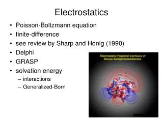
Electrostatics
Electrostatics. Electrostatics. Electrostatics. An electrostatic field is produced by a static (or time-invariant) charge distribution. A field produced by a thunderstorm cloud can be viewed as an electrostatic field. .

Electrostatics
E N D
Presentation Transcript
Electrostatics Electrostatics An electrostatic field is produced by a static (or time-invariant) charge distribution. A field produced by a thunderstorm cloud can be viewed as an electrostatic field. Coulomb’s law deals with the force a point charge exerts on another point charge. The force Fbetween two charges Q and Q is 1. Along the line joining Q and Q 2. Directly proportional to the product Q Q of the charges 3. Inversely proportional to the square of the distance r between the charges 1 2 1 2 1 2
Electrostatics In the international system of units (SI), Q and Q are in coulombs (1C is approximately equivalent to electrons since one electron charge e = C), the distance r is in meters, and the force F is in newtons so that: 1 2 the permittivity of free space F/m m/F or
Electrostatics Electric field intensity (or electric field strength) is defined as the force per unit charge that a very small stationary test charge experiences when it is placed in the electric field. , In practice, the test charge should be small enough not to disturb the field distribution of the source. For a single point charge Q located at the origin where is a unit vector pointing in the radial direction (away from the charge). is valid for vacuum and air. For other materials should be replaced by (typically ).
Electrostatics Suppose that there are several charges located at positions with respect to the origin. The observation point is at position . The vector from the ith charge to the observation point is ( ), and the distance is . Source point The total field due to N charges is Observation (field) point
Electrostatics Example: Find the electric field at P due to Q and –Q. The vector from Q to P lies in the x-y plane. Therefore, (the z component of ) vanishes at P. y components due to Q and –Q are equal and opposite and therefore add to zero. Thus, has only an x component.
Electrostatics Charge density Various charge distributions. Consider a charged wire. Charge on an elemental wire segment is so that the charge per unit length . The total electric field is the sum of the field contributions from the individual segments. If we let we get Position of the field point Position of the source point
Electrostatics If the charge is distributed on a surface (surface charge density ), we can write Surface integral Unit vector directed from the source point to the field point If charge is distributed through a volume , Integral over the volume containing the charge
Electrostatics Example: A circular disk of radius b with uniform surface charge density , lies in the x-y plane with its center at the origin. Find the electric field at P (z=h). All the contributions in the x and y directions are cancelled, and the field at P contains only z component.
Electrostatics The Source Equation As we have seen, the electric field can be expressed as an integral of the charges that produce it. The charge can be expressed in terms of derivatives of the electric field: source equation divergence operator Let Then scalar
Electrostatics The Source Equation continued Example: Let be the field of a single point charge Q at the origin. Show that is zero everywhere except at the origin. where The x component of is The divergence of a vector field at a given point is a measure of how much the field diverges or emanates from that point. except at the origin (x=0,y=0,z=0) where the derivatives are undefined.
Electrostatics The Source Equation continued In cylindrical coordinates In spherical coordinates Example: Let be the electrostatic field of a point charge Q at the origin. Express this field in spherical coordinates and find its divergence. everywhere except at the origin, where is undefined (because the field is infinite).
Electrostatics Gauss’ Law Essentially, it states that the net electric flux through any closed surface is equal to the total charge enclosed by that surface. Gauss’ law provides an easy means of finding for symmetrical charge distributions such as a point charge, an infinite line charge, and infinite cylindrical surface charge, and a spherical distribution of charge. Let us choose an arbitrary closed surface S. If a vector field is present, we can construct the surface integral of over that surface: The total outward flux of through S The divergence of (a scalar function of position) everywhere inside the surface S is .We can integrate this scalar over the volume enclosed by the surface S. Over the volume enclosed by S
Electrostatics Gauss’ Law continued According to the divergence theorem We now apply the divergence theorem to the source equation integrated over the volume v: Gauss’ Law the angle between and the outward normal to the surface Gaussian surface - the normal component of
Electrostatics Gauss’ Law continued Example: Find the electric field at a distance r from a point charge q using Gauss’ law. Let the surface S (Gaussian surface) be a sphere of radius r centered on the charge. Then and . Also (only radial component is present). Since Er = constant everywhere on the surface, we can write
Electrostatics Gauss’ Law continued Example: A uniform sphere of charge with charge density and radius b is centered at the origin. Find the electric field at a distance r from the origin for r>b and r<b. As in previous example the electric field is radial and spherically symmetric. (1) r > b decreases as (2) r < b increases linearly with r Gauss’ law can be used for finding when is constant on the Gaussian surface.
Electrostatics Gauss’ Law continued Example: Determine the electric field intensity of an infinite planar charge with a uniform surface charge density . coincides with the xy-plane The field due to a charged sheet of an infinite extent is normal to the sheet. We choose as the Gaussian surface a rectangular box with top and bottom faces of an arbitrary area A, equidistant from the planar charge. The sides of the box are perpendicular to the charged sheet.
Electrostatics Gauss’ Law continued On the top face On the bottom face There is no contribution from the side faces. The total enclosed charge is
Electrostatics Ohm’s Law Ohm’s law used in circuit theory, V=IR, is called the “macroscopic” form of Ohm’s law. Here we consider “microcopic” (or point form). (Applicable to conduction current only). Let us define the current density vector . Its direction is the direction in which, on the average, charge is moving. is current per unit area perpendicular to the direction of . The total current through a surface is (if , , , ) According to Ohm’s law, current density has the same direction as electric field, and its magnitude is proportional to that of the electric field: where is the electric conductivity. The unit for is siemens per meter ( ). Copper S/m Seawater 4 S/m Glass S/m
Electrostatics Ohm’s Law continued The reciprocal of is called resistivity, in ohm-meters ( ). Suppose voltage V is applied to a conductor of length l and uniform cross section S. Within the conducting material ( constant) “macroscopic” form of Ohm’s law Resistance of the conductor
Electrostatics Electrostatic Energy and Potential A point charge q placed in an electric field experiences a force: If a particle with charge q moves through an electric field from point P1 to point P2, the work done on the particle by the electric field is This work represents the difference in electric potential energy of charge q between point P1 and point P2 W = W - W 1 2 (W is negative if the work is done by an external agent) The electric potential energy per unit charge is defined as electric potential V (J/C or volts) Electrostatic potential difference or voltage between P and P (independent of the path between P and P ) 1 2 1 2
Electrostatics Electrostatic Energy and Potential continued V1and V2 are the potentials (or absolute potentials) at P1 and P2, respectively, defined as the potential difference between each point and chosen point at which the potential is zero (similar to measuring altitude with respect to sea level). In most cases the zero–potential point is taken infinity. Example: A point charge q is located at the origin. Find the potential difference between P1 (a,0,0) and P2 (0,b,0) due to q is radial. Let us choose a path of integration composed of two segments. Segment I (circular line with radius a) and Segment II (vertical straight line).
Electrostatics Electrostatic Energy and Potential continued Example continued: Segment I contributes nothing to the integral because is perpendicular to everywhere along it. As a result, the potential is constant everywhere on Segment I; it is said to be equipotential. On Segment II, , , and If we move P2to infinity and set V2=0, where a is the distance between the observation point and the source point for line charge for surface charge In general, for volume charge
Electrostatics Gradient of a Scalar Field By definition, the gradient of a scalar field V is a vector that represents both the magnitude and direction of the maximum space rate of increase of V. The gradient operator is a differential operator. It will act on the potential (a scalar) to produce the electric field (a vector). Let us consider two points and which are quite close together. If we move from P1 to P2 the potential will change from V to where 1 due to the change in z scalar The displacement vector (express the change in position as we move from P1and P2) is vector
Electrostatics Gradient of a Scalar Field continued The relation between and can be expressed using the gradient of V: vector On the other hand, if we let P1 and P2 to be so close together that is nearly constant, (potential difference equation) The negative sign shows that the direction of is opposite to the direction in which V increases.
Electrostatics Gradient of a Scalar Field continued Example: Determine the electric field of a point charge q located at the origin, by first finding its electric scalar potential.
Gradient of a Scalar Field continued Example continued: Determine the electric field of a point charge q located at the origin, by first finding its electric scalar potential. vector the angle between and points in the direction of the maximum rate of change in V. at any point is perpendicular to the constant V surface which passes through that point (equipotential surface). (V=const)
Electrostatics Gradient of a Scalar Field continued The electric field is directed from the conductor at higher potential toward one at lower potential. Since , is always perpendicular to the equipotentials. If we assume that for an ideal metal , no electric field can exist inside the metal (otherwise , which is impossible). Considering two points P1 and P2 located inside a metal or on its surface – and recalling that we find that V1=V2. This means the entire metal is at the same potential, and its surface is an equipotential. For cylindrical coordinates For spherical coordinates
Electrostatics Capacitors Any two conductors carrying equal but opposite charges form a capacitor. The capacitance of a capacitor depends on its geometry and on the permittivity of the medium. The capacitance C of the capacitor is defined as the ratio of the magnitude of Q of the charge on one of the plates to the potential difference V between them. Area A d d isvery small compared with the lateral dimensions of the capacitor (fringing of at the edges of the plates is neglected) A parallel-plate capacitor. Cylindrical Gaussian Surface Top face (inside the metal) Side surface Bottom face Close-up view of the upper plate of the parallel-plate capacitor.
Electrostatics Laplace’s and Poisson’s Equations The usual approach to electrostatic problems is to begin with calculating the potential. When the potential has to be found, it is easy to find the field at any point by taking the gradient of the potential the divergence operator the source equation vector the gradient operator the Laplacian operator Poisson’s equation scalar If no charge is present , Laplace’s equation
Electrostatics Laplace’s and Poisson’s Equations continued The form of the Laplacian operator can be found by combining the gradient and divergence operators. - in rectangular coordinates - in cylindrical coordinates • in spherical • coordinates Electrostatic problems where only charge and potential at some boundaries are known and it is desired to find and V throughout the region are called boundary-value problems. They can be solved using experimental, analytical, or numerical methods.
Electrostatics Method of Images A given charge configuration above an infinite grounded perfectly conducting plane may be replaced by the charge configuration itself, its image, and an equipotential surface in place of the conducting plane. The method can be used to determine the fields only in the region where the image charges are not located. Original problem Construction for solving original problem by the method of images. Field lines above the z=0 plane are the same in both cases. By symmetry, the potential in this plane is zero, which satisfies the boundary conditions of the original problem.