Download
1 / 20
210 likes | 720 Vues
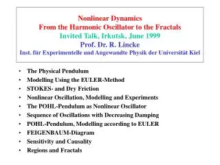
Nonlinear Dynamics From the Harmonic Oscillator to the Fractals Invited Talk, Irkutsk, June 1999 Prof. Dr. R. Lincke Inst. für Experimentelle und Angewandte Physik der Universität Kiel. The Physical Pendulum Modelling Using the EULER-Method STOKES- and Dry Friction

E N D
Nonlinear DynamicsFrom the Harmonic Oscillator to the FractalsInvited Talk, Irkutsk, June 1999Prof. Dr. R. LinckeInst. für Experimentelle und Angewandte Physik der Universität Kiel • The Physical Pendulum • Modelling Using the EULER-Method • STOKES- and Dry Friction • Nonlinear Oscillation, Modelling and Experiments • The POHL-Pendulum as Nonlinear Oscillator • Sequence of Oscillations with Decreasing Damping • POHL-Pendulum, Modelling according to EULER • FEIGENBAUM-Diagram • Sensitivity and Causality • Regions and Fractals
The Harmonic OscillatorApproximated by a Physical Pendulum If one uses a potentiometer as transducer, the damped oscillation recorded does not show the expected exponential damping.
Damped OscillationsModelling Using the EULER-Method A) Stokes‘ Friction B) Dry Friction
Physical Pendulum With Low FrictionTransducer: Hall Probe A) Stokes‘ Friction B) Dry Friction
LC OscillationsMeasuring Frequency andDecay Constant R L = 7,34 mH = 787,1 Hz C = 5,57 µF T = 1,27 ms RL = 4,2 = RL/2L = 286/s R = 1 M ADW C L (RL) Contrary to the mechanical oscillations, here the agreement between experiment and theory is excellent.
Nonlinear OscillationsModelling with the EULER-Method If one adds a term in x4 to the parabolic potential of a harmonic oscillator (i.e. a cubic term to the linear force), one ends up with a DUFFING-Potential. The resulting oscillation shows the typical behaviour: For nonlinear oszillators the period depends on the amplitude!
Nonlinear Mechanic Oscillations Some Other Experimental Setups B) Physical Pendulum With Large Angles A) Airtrack Decke Schraubenfeder At 90° initial angle, the period is already 18% longer than at 5° Umlenkstift F ~ x 3 Bahn C) Double Pendulum Period as Function of Initial Angle theory/experiment
WackelschwingerA Nonlinear Oscillator Induction Coils Characteristics of a NonlinearOscillator: The time function is not harmonic. The period depends on the amplitude.
POHL Pendulum With Excentric MassParadigm for a Nonlinear Oscillator Position Transducer BMW BMW Unwucht Schrittmotor PC-Interface Wirbelstrombremse The wellknown POHL Pendulum is a typical harmonic Oscillator used for demonstration purposes. With added excentric mass and a stepper motor it became a paradigm for the nonlinear oscillator.
POHL PendulumDuffing-Potential The added excentric mass transforms the parabolic potential of the harmonic POHL Pendulum into a DUFFING potential with ist characteristic two minima. Vd()=V()+D·(1+cos)+C V()=½k·² By setting the eddy current damping accor-dingly, the following modes can be realized: 0: free oscillation, only mechanical friction 1: strong damping, quasi-harmonic 2: lesser damping, period doubling 3: lesser damping, period quadrupling 4: very low damping, chaos These four modes of oscillation are now investigated experimentally and with appropriate modelling. 0 4 3 2 1
POHL PendulumPosition Transducer BMW Figures: The diagrams show the angle as function of time, the velocity as function of time and the velocity as function of angle (phase space). Left: No eddy current brake, only mechanical damping, no motor excitation. The pendulum was started in the extreme right position; it ends in the right potential minimum. Right: Excitation by stepping motor excenter, strong eddy current damping. The oscillation is nearly harmonic, the phase diagram is similar to an ellipse. 0 1
POHL PendulumPosition Transducer BMW Figures: In the diagrams angle as function of time and velocity as function of time, the motor phase is shown in addition. Left: The amplitudes of the oscillation alternate. One complete period of oscillation corresponds to two periods of the motor; this is called Period Doubling. Right: Four motor periods correspond to one complete oscillatory period. 2 3
POHL PendulumModelling with the EULER-Method Equation of motion: ·d2/dt2 = - k· - ·d/dt + A·cos(·t) -T·sin() Abbreviations: Phi = , Phi1 = d/dt, Phi2 = d2/dt2 Torque caused by added excentric mass. t := 0; Phi := 0; Phi1 := 0; REPEAT EULER-Method t := t + dt; Phi2 := - k/ ·Phi - / ·Phi1 + A/ · cos(·t) -mgR/ ·sin(); Phi1 := Phi1 + Phi2 ·dt; Phi := Phi + Phi1 ·dt; PutPixel (round(t),round(100-20·Phi),1); UNTIL t>639; In order to study further phenomena, we now continue with modellings of POHL Pendulumusing the algorithm shown here:
POINCARÉ SectionAn Alternative Representation For chaotic oscillations, neither the time function x(t) nor the phase diagram v(x) are very illuminating. Quite often deeper systematics appear, if one uses the phase diagram and marks those points that belong to a certain phase of the motor excitation (quasi ‘stroboscopically‘): such a representation is called Poincaré Section. The diagram on the left shows an oscillation with doubled period and thus two different Poincaré points. With period quadrupling, there would be four points and chaotic oscillations would show an infinite number. Often the Poincaré points assemble on marked trajectories, the socalled Strange Attractors.
POHL PendulumModelling with the EULER Method This program reproduces all measure-ments with the POHL Pendulum and the BMW transducer. Representative are the three aspects of a period quadrupling shown here. Time Function Phase Space 4 Poincaré Points
POHL PendulumModelling with the EULER Method If the damping is decreased even further, the behaviour of the pendulum becomes chaotic:The time function shows no periodicity, and in the phase diagram the whole space is filled; the Poincaré points, however, gather in a ‘strange attractor‘ Phase Space Poincaré Points
POHL PendulumModelling with the EULER Method A systematic variation of the damping yields the socalled Feigenbaum Diagram. This plot here shows 100 extrema (max and min) after a transient period of 300 seconds. The marked positions correspond to the oscillatory modes shown before: 1. Simple oscillation. 2. Period doubling. 3. Period quadrupling. 4. Chaos. 5. Window in Chaos. 6. Free oscillation. 1 2 3 6 4 5
Sensitivity Towards Initial ConditionsCausality and Deterministisc Chaos This picture shows the initial oscillations with starting angles of 50° and 50,2°. In the very beginning, no difference is visible. Close to the central maximum of the potential, the curves begin to separate, and soon they are completely different. The red trace gives the logarithm of their distance in phase space, i.e. log(x1-x2)²+(v1-v2)² : the curves diverge exponentially. • Weak Causality: Equal causes have equal effects. • Strong Causality: Similar causes have similar effects. • Deterministic Chaos: The sensitivity prevents long term predictions.
Sensitivity Towards Initial Conditionso: 135.550°, 135.560°, 135.563° Even a very slight variation in the initial conditions can result in completely different oscillations. In the upper two pictures, the oscillations stabilize in the right half of the pendulum, in the left picture in the left half. A systematic investigation (varying the initial velocity also) produces two dimensional Domains for reaching stable oscillations in the right or left half of the POHL pendulum.
POHL Pendulum Domains for Settling in the Left/Right Half Repeated ZOOM:Self Similarity