Introduction to Probability: Understanding Events, Outcomes, and Measurement
This introduction explores the fundamentals of probability, emphasizing the concepts of events, outcomes, and sample spaces. We discuss the process of quantification in science, defining key terms such as trials, experiments, and the nature of random versus deterministic processes. The mathematical foundations of probability are established through axioms and examples, illustrating how to calculate the probability of simple and complex events. Furthermore, we analyze independence among events and provide real-world scenarios, including whirligig beetles, to demonstrate probability calculations.

Introduction to Probability: Understanding Events, Outcomes, and Measurement
E N D
Presentation Transcript
Introduction to Probability The problems of data measurement, quantification and interpretation
Event It is a simple process with a well-recognized beginning and end
Outcome One of the alternatives through which an event manifests
Sample space The set formed from all possible outcomes of an event
Trial • A single complete instance of a process of testing • Statisticians refer to each trial as an individual replicate, and refer to a set of trials as an experiment
Probability • Most statistics textbooks define probability just as we have done: the (expected) frequency with which events occur
An example of a trial: flipping a coin…An example of an experiment: flipping a coin several times...Sample space: {heads} {tails} ...
Random and Deterministic processes • When we say that events are random, stochastic, probabilistic, or due to chance, what we really mean is that their outcomes are determined in part by a complex set of processes that we are unable or unwilling to measure and will instead treat as random • The strength of other processes that we measure, manipulate, and model represent deterministic or mechanistic forces
The mathematics of Probability • Axiom 1: the sum of the probabilities of outcomes within a single sample space =1.0 • In a properly defined sample space the outcomes are mutually exclusive and exhaustive
The whirligig beetle These beasts always produce exactly two litters, with between 2 and 4 offspring per litter
The lifetime reproductive success of a beetle can be described as an outcome (a,b) where a represents the number of offspring in the first litter and b the number of offspring in the second litter
The sample space Whirligig BeetleFitness consists of all possible lifetime reproductive outcomes: • Fitness = {(2,2),(2,3),(2,4) (3,2),(3,3),(3,4) (4,2),(4,3),(4,4)} P(2,2)=P(2,3)=P(2,4) = … =P(4,4) 1/9+1/9+1/9+1/9+1/9+1/9+1/9+1/9+1/9=1
Complex events • Are composites of simple events in the sample space • A complex event can be achieved by one of several pathways (OR statement) • Event A or Event B orEvent C, represented by the union of simple events (A U B U C)
Complex events: summing probabilities • What is the probability that a whirligig beetle produces 6 offspring? • 6 offspring ={(2,4),(3,3),(4,2)} Fitness (2,2) (2,3) (4,2) (3,4) (2,4) (4,3) (3,2) (4,4) (3,3) 6 offspring
Complex events • Axiom 2: the probability of a complex event equals the sum of the probabilities of the outcomes that make up that event • P (6 offspring) = P(2,4) or P(3,3) or P(4,2) = 1/9+1/9+1/9 = 3/9 = 1/3 • P(A or B or C)= P(A)+P(B)+P(C)
Shared events • Are multiple simultaneous occurrences of simple events in the sample space • A shared event requires the simultaneous occurrence of two or more simple events (AND statement) • Event A and Event B andEvent C, represented by the intersection of simple events (A ∩ B ∩ C)
Shared events: multiplying probabilities • If, instead, we assume the number of offspring produced in the second litter is independent of the number produced in the first litter • Suppose that an individual can produce 2,3,4 offspring in each litter and that the chances of each of these events are 1/3. • What is the probability of obtaining the pair of litters (2,4)? • 2,4 offspring ={(2,4)}
Independence • Two events are independent of one another if the outcome of one event is not affected by the outcome of the other • If two events are independent of one another, then probability that both events occur (a shared event) equals the product of their individual probabilities
If A and B are independent 1/3*1/3=1/9 Fitness (2) (4) (2) (4) (3) (3) First litter Second litter
Probability calculations • Imagine two kinds of milkweed populations: those that evolved secondary chemicals that make them resistant (R) to the herbivore, and those that haven’t (not R) • Suppose you census a number of milkweed populations and determine that 20% of the populations are resistant to the herbivore • Thus P(R)=0.20; P(not R)=0.80
Probability calculations • Similarly, suppose that the probability that the caterpillar (C) occurs in a patch is 0.7 • Then P(C)=0.7; P(not C)=0.3. • If colonization events are independent of one another, What are the chances of finding either caterpillars, milkweeds, or both in these patches? • What is the probability that the milkweed will disappear?
Notice • 0.24+0.56+0.06+0.14=1 • 0.14+0.06=0.20 (probability of resistance) • 0.56+0.14=0.70 (probability of caterpillar presence) • 0.56 Probability that milkweed will disappear
Rules for combining sets when events are not independent • Suppose in our sample space there are two identifiable events, each of which consists of a group of outcomes: 1. whirligig that produces exactly 2 offspring in the first litter (F) 2. whirligig that produces exactly 4 offspring in the second litter (S)
Rules for combining sets when events are not independent • Fitness={(2,2),(2,3),(2,4) (3,2),(3,3),(3,4) (4,2),(4,3),(4,4)} F={(2,2),(2,3),(2,4)} S={(2,4),(3,4),(4,4)} F={(2,2),(2,3),(2,4)} S={(2,4),(3,4),(4,4)}
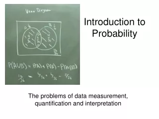
Venn diagram Fitness F (2,2) (2,3) (2,4) (4,2) (3,4) S (4,4) (3,2) (4,3) (3,3)
Rules for combining sets when events are not independent • We can construct a third useful set by considering the set Fc , called the complement of F, which is the set of objects in the remaining sample space • Fc={(3,2),(3,3),(3,4),(4,2),(4,3),4,4)} • From axioms 1 and 2: P(F)+P(Fc)=1
= Empty set • The empty set contains no elements and is written as
Calculating probabilities of combined events If: then: ={ }
How to estimate the probability that a whirligig produces 6 offspring, if the number of offspring produced in the second litter depends on the number of offspring in the first litter? • Recall the complex event 6 offspring is P(6 offspring) = {(2,4),(3,3),(4,2)} = 3/9 (or 1/3) • If you observed that the first litter was 2 offspring, what is the probability that the whirligig will produce 4 offspring next time? Answer = 1/3 is correct, but why??????
Conditional probabilities • If we are calculating the probability of a complex event, and we have information about the outcome of that event, we should modify our estimates of the probabilities of other outcomes accordingly. We refer to these updated estimates as conditional probabilities P(A│B) or the probability of event A given event B
The probability of A is calculated assuming that the event B has already occurred:
Rearranging the formula gives us a general formula for calculating the probability of an intersection: Note that if two events A and B are independent, then P(A|B)=P(A), so that
The frequentist paradigm • Until now, we have discussed probability using what is know as the frequentist paradigm, in which probabilities are estimated as the relative frequencies of outcomes based on an infinitely large set of trials • Scientists start assuming NO prior knowledge of the probability of an event, and re-estimate the probability based on a large number of trials
Bayes’ Theorem • In contrast is the Bayesian paradigm, which builds on the idea that investigators may already have a belief about the probability of an event, before the trials are conducted. • These prior probabilities may be based on previous experience, intuition, or model predictions • These prior probabilities are then modified by the data from the current trial to yield posterior probabilities.
Bayes’ Theorem The probability of an event or outcome A conditional on another event B can be determined if you know the probability of the event B conditional on the event A and you know the complement of A
An important distinction • For example, the distinction between: • P(C|R), the probability that caterpillars are found given a resistant population of milkweeds. To estimate P(C|R), we would need to examine populations of resistant milkweeds to determine the frequency with which these populations were hosting caterpillars
An important distinction • and: • P(R|C), the probability that milkweeds are resistant given that they are eaten by caterpillars. To estimate P(R|C), we would need to examine caterpillars to determine the frequency with which their host plants are resistant.
Probability is completely contingent on how we define the sample space • In general, we all have intuitive estimates for probabilities for all kinds of events. • However, to quantify those guesses, we have to decide on a sample space, take samples, and count the frequency with which certain events occur
Estimating probability by sampling • We can efficiently estimate the probability of an event by taking a sample of the population of interest Exercise 1 Part 1, with cards
Estimating probabilities by sampling • Using playing cards identify Kings, Queens, Jacks and Aces as “captures”, and the rest of the cards as “non captures”. • What is the probability of “capture”? • Shuffle to provide an element of chance in the game. • Take at random four cards and note how many of them are “captures” • Repeat this procedure (Steps 3. and 4.) 20 times • What is the expected value of the capture probability? students will have one week to complete this exercise
Estimating probabilities by sampling • Do the same exercise, but use only the heart suit • What is the expected value of the capture probability? • How different is the result among the games you played?
Exercise 1 Part 2, A model of the game • Write an algorithm (sequence of instructions) in Excel that simulates the game previously described (be creative) • Play the game 10 and 20 times • How different are the results from the games you played? (present the results as histograms) • What is the expected value of the capture probability?
Example of Histogram • The numbers on the horizontal axis, or x-axis indicate the number of “captures” • The numbers on the vertical axis or y-axis indicate the frequency

