Download
1 / 73
730 likes | 1.03k Vues
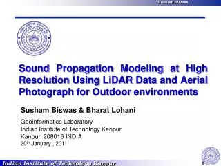
Sound Propagation Modeling at High Resolution Using LiDAR Data and Aerial Photograph for Outdoor environments. Susham Biswas & Bharat Lohani Geoinformatics Laboratory Indian Institute of Technology Kanpur Kanpur, 208016 INDIA 20 th January , 2011.

E N D
Sound Propagation Modeling at High Resolution Using LiDAR Data and Aerial Photograph for Outdoor environments Susham Biswas & Bharat Lohani Geoinformatics Laboratory Indian Institute of Technology Kanpur Kanpur, 208016 INDIA 20th January , 2011
Representation of Outdoor Sounds and/or its applications Noise map Around Airport Animation Videography-movie Impulsive sound propagation i.e., gun shot, bomb blast etc Urban Noise Map (e.g., UK Noise Map)
Outdoor Sounds and its Relationship with Spatial and other Data : Modeling aspect
Sound modeling Sound Modeling Sound Input Spatial Parameter Sound Model Sound Output
Outdoor Sound Propagation Transmitted Wave Sound Absorbed Wave Reflector Obstruction Diffracted Wave Reflected Wave Ground Ground Reflected Wave
Sound Modeling • Numerical Modeling • Classical Wave Equation Solutions • Approximate Wave Equation Solutions • Diffracted Sound Field Determination Techniques • Boundary Element Method • Empirical or Semi-Empirical Modeling –It has the following components • Directivity • Distance Attenuation • Atmospheric Attenuation • Ground Attenuation • Barrier Attenuation • Barrier_ground attenuation • Meteorological Correction • Vegetative Attenuation • Reflection Correction
Sound Modeling (Semi_emperical) How sound can reach receiver R from source PS Direct Transmission Direct transmission of sound from source to receiver
How sound can reach receiver R from source PS Ground Reflected Sound transmission after ground reflection
Diffracted over and around sides of building How sound can reach receiver R from source PS
How sound can reach receiver R from source PS Wall reflected Transmission through reflection from wall
How sound can reach receiver R from source PS Tree absorbed
Spatial information required in sound modeling !! In outdoor environment sound from a source follows one or many of the above paths before reaching to a receiver location thus the outdoor Sound propagation involves following spatial parameters Distance between Source* (PS) and Receiver (R) Path_difference for Diffraction Path for Ground_reflection with ground type Possibility of Wall_reflection Extent of path length involved in tree_absorption * When there exists objects between Source and receiver the intermediate diffracting, reflecting points involved in transmission is termed as secondary source (SS) and original source as primary source (PS)
Poor Sound Model Sound model (Important components) Distance attenuation Building attenuation Spatial Parameter Where N: Fresnel Number Atmospheric attenuation
Poor Sound Model Sound model (Important components) Ground attenuation 3 Zone approach (ISO-9613-2) Complex approach Ground reflecting point dependent Spatial Parameter Tree attenuation
Existing practices Existing scenario: In Spatial Data and its Input Techniques-Weaknesses • Spatial Input using • Approximate Techniques (e.g Spot Heights) • Contour • Vector based Approach (e.g., Map Digitization) • Accurate Comprehensive Surveying (time limitation) Spatial Data • Approximate estimation of terrain heights • Low resolution satellite image/ aerial photo • Use of Total Station/GPS in limited scale
Objectives of research Can Lidar data be used for sound modeling- how? Is there any Advantage of using high resolution spatial data? Whether Better Data and/ or Model can lead to better prediction?
Prediction of Sound at Outdoor with Poor Data and Poor Model Observed Sound at outdoor Prediction of Sound at Outdoor with Good Data and Poor Model Comparison Can LiDAR data & Aerial Photograph be used for Sound Modeling? Prediction of Sound at Outdoor with Good Data and Good Model Field Measurement Sound Prediction Schemes • Is there any Advantage of using high resolution spatial data? • Whether Better Data and/ or Model can lead to better prediction? • Can better data suggest ways of improvement in sound modeling? • Methodology
Methodology • Field Measurement • Sound Measurement • Spatial data Measurement • Non_Spatial data Measurement • Sound Prediction Schemes • Poor Data and Poor Model • Good Data and Poor Model • Good Data and Good Model • Comparative Analysis
Spatial Survey Design of Algorithms Design of Model Spatial Parameters Measured Field Data Sound Parameters at Source Predicted Sound for outdoor location Sound Model Non-Spatial Parameters Measured Field Data • Sound Prediction Scheme Methodology Contd.
Design of Algorithm to extract Spatial Parameters • Data Preparation For Good data: Accurate Data e.g. from Total Station, or LiDAR and Aerial Photographic Survey etc For Poor data: Errors added to good data
How to do LiDAR data points Building points Ground points Tree points Classification Triangulation / cluster formation/ Other Building corner points and building edges Ground TIN TIN from tree points cluster Coordinates of source and receiver Determination of principal propagation paths Cutting plane technique Modeling parameters Ground type attribute Classified aerial photo Sound Model Receiver sound level Source sound level
Aim Determination of all principal paths for propagation
Determination of Principal Path due to diffraction (over top)
Determination of Principal Path due to diffraction (over top) Cutting plane technique Cutting plane orthogonal to X-Y plane and passing through source and receiver
Determination of Principal Path due to diffraction (over top) Intersecting points Intersecting points with vertical line of intersection between buildings and cutting plane Intersecting points & vertical line of intersection
Determination of Principal Path due to diffraction (over top) Finding effective intersecting points
Determined of Principal Path due to diffraction (over top) Determined principal path over top (i.e., PS-c-d-R)
Determination of Principal Path due to diffraction (around sides) Cutting plane technique
Determination of Principal Path due to diffraction (around sides) Intersecting points at cutting plane
Determination of Principal Path due to diffraction (around sides) Intersecting points & line of intersection Intersecting points and line of intersection between building side walls and cutting plane
Determination of Principal Path due to diffraction (around sides) Intersection points with projected lines of intersection Intersecting points and lines of intersection projected on XY plane
e Determination of Principal Path due to diffraction (around sides) h a d g f b c Principal paths around sides (i.e., PS-a-e-h-R and PS-b-c-R)
Eight Principal path or routes between any pair of Source and Receiver Source 5 & 6 Source Receiver 1 Source Receiver 2 Receiver Source Source Receiver 3 7 & 8 Source Receiver 4 Receiver
Determination of Principal Path for ground reflection Comparison of TIN planes with PS-R vertical plane Classified ground point Triangulation
Determination of Principal Path stretch causing tree absorption Finding TIN planes intersected by PS-R line Classified tree points K-Mean clustering Triangulation
Finding the point of reflection (if any) Reflecting Point Source Receiver The plane of “Source – Reflecting Point – Receiver” The plane of “Wall”
Spatial Data Prediction Scheme with Poor Model Dist S-R Path-Diff Avg. Gr.Type Predic ted SPL ) = ( AAtm + - + AB AG + SPLS AD
Prediction Scheme with Good Model1 Spatial Data • Dist S-R • Path-Diff w.r.t. 8 Principal routes • Gr. Type of ground reflecting point • Angles of reflections • Phase change at reflection • Shape of Barrier • Turbulency Factors Aveg. AR AD . . . . . . Coherent ABG . . . Predicted SPL - . SPLS = + + + + + + + + + + 1DI 1AD 1ABG 1AAtm 1AR 1Aveg. 8DI 8AD 8ABG 8AAtm 8AR 8Aveg.
Prediction Scheme with Good Model2 Spatial Data Dist S-R Path-Diff w.r.t. 8 Principal routes Gr. Type of ground reflecting point Angles of reflections Phase change at reflection Shape of Barrier Turbulency Factors Aveg. AR AD . . . Incoherent . . . ABG . . . Predicted SPL - . SPLS = + + + + + + + + + + 1DI 1AD 1ABG 1AAtm 1AR 1Aveg. 8DI 8AD 8ABG 8AAtm 8AR 8Aveg.
Design of Experiment Experimental Setups Sound Generation Sound Measurement Position Measurement Experimental Parameters • Frequency of sound • SPL/Leq • Experimental Schedule • Experiment • Primary Experiment • Auxiliary Experiment
Validation experiment A transact (130mX 30 m) at IIT Kanpur Air strip containing building, different ground types, tree, is used to monitor SPL and validate that with developed model
Propagated Sound Measured Sound at Receiver Spatial Survey Experiment-Measurement of Sound and Spatial data Reflector for TS Measured Sound at Source Total Station
Experimental Detail- Sound Generation Computer (Generation of Tonal Sound) Speaker (output device) Amplifier
Experimental Detail- Sound Measurement (at receiver) Sound Measured simultaneously at a fixed position at source as well
Measured SPL in dB dB Frequency=250Hz
Predicted SPL in dB (for Good data and Good Model1) dB Frequency=250Hz
Deviation between measured & predicted Good data – Good Model1 -250 Hz Deviation in dB
Deviation between measured & predicted Good data – Good Model1 500 Hz Deviation in dB
Deviation between measured & predicted Good data – Good Model1 1000 Hz Deviation in dB