Download
1 / 17
540 likes | 1.64k Vues
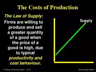
The Costs of Production. The Law of Supply : Firms are willing to produce and sell a greater quantity of a good when the price of a good is high, due to typical productivity and cost behaviour. Supply. Total Revenue, Total Cost, Profit.

E N D
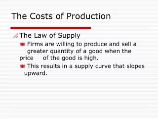
The Costs of Production The Law of Supply: Firms are willing to produce and sell a greater quantity of a good when the price of a good is high, due totypical productivity and cost behaviour. Supply
Total Revenue, Total Cost, Profit • We assume that the firm’s goal is to maximize profit. Profit = Total revenue – Total cost TR-the amount a firm receives from the sale of its output TC-the market value of the inputs a firm uses in production
Costs as Opportunity Costs • The firm’s costs include Explicit Costs and Implicit Costs: • Explicit Costs: costs that involve a direct money outlay for factors of production. • Implicit Costs: costs that do not involve a direct money outlay (e.g. opportunity costs of the owner’s own inputs used - implicit wages, implicit rent, cost of capital).
Costs as Opportunity Costs • Accountants measure the explicit costs but often ignore the implicit costs. • Economists include all opportunity costs when measuring costs. • Accounting Profit = TR - Explicit Costs • Economic Profit = TR - Explicit Costs - Implicit Costs
Explicit vs. Implicit Costs: An Example You need $100,000 to start your business. The interest rate is 5%. • Case 1: borrow $100,000 • explicit cost = $5000 interest on loan • Case 2: use $40,000 of your savings, borrow the other $60,000 • explicit cost = $3000 (5%) interest on the loan • implicit cost = $2000 (5%) foregone interest you could have earned on your $40,000. In both cases, total (exp+ imp) costs are $5000.
Marginal Product • The marginal productof any input is the increase in output arising from an additional unit of that input, holding all other inputs constant. • E.g., if Farmer Jack hires one more worker, his output rises by the marginal product of labour. • Notation: ∆ (delta) = “change in…” Examples: ∆Q = change in output, ∆L = change in labour • Marginal product of labour (MPL) = delta Q/delta L
Why MPL Diminishes • Diminishing marginal product: the marginal product of an input declines as the quantity of the input increases (other things equal) E.g., Farmer Jack’s output rises by a smaller and smaller amount for each additional worker. Why? • If Jack increases workers but not land, the average worker has less land to work with, so will be less productive. • In general, MPL diminishes as L rises whether the fixed input is land or capital (equipment, machines, etc.).
Short-Run vs. Long-Run Two different time horizons are important when analyzing costs. • Short-Run: Time period over which some inputs are variable (labour, materials) and some inputs are fixed (plant size). • Long-Run: Time period over which all inputs are variable, including plant size.
Short-Run Costs Costs of production may be divided into two categories in the short-run: • Fixed Costs: • Those costs that do not vary with the amount of output produced. • Variable Costs: • Those costs that do vary with the amount of output produced.
Marginal Cost • Marginal Cost (MC) is the increase in Total Cost from producing one more unit: • MC = delta TC/delta Q
The Shape of Short-Run Cost Curves • Short-run cost behaviour is based on the productivity of the inputs (resources). • As the firm continues to expand output,in a fixed plant-size situation, eventuallythe marginal product of each successive worker hired will decrease. • The diminishing marginal product causesthe marginal cost to increase in the short-run. This in turn affects the behaviour of average total cost.
The Shape of Typical Cost Curves U-Shaped Average Total Cost (ATC): • At low levels of output, as the firm expands production, ATC declines. • At higher production levels, as output is increased, ATC increases. • The bottom of the U-Shape occurs at the quantity that minimizes average total cost. • This is called the Efficient Sizeof the firm.
The Relationship Between Marginal Cost and Average Total Cost • Why is ATC U - shaped? • When marginal cost is less than average total cost, average total cost is falling. MC < ATC ATC • When marginal cost is greater than average total cost, average total cost is rising. MC > ATC ATC
The Relationship Between Marginal Cost and Average Total Cost MC ATC Cost ($’s) The marginal cost curve always crosses the average total cost curve at the minimum average total cost! Quantity
Costs in the Short Run & Long Run • Short run: Some inputs are fixed (e.g., factories, land). The costs of these inputs are FC. • Long run: All inputs are variable (e.g., firms can build more factories, or sell existing ones) • In the long run, ATC at any Q is cost per unit using the most efficient mix of inputs for that Q (e.g., the factory size with the lowest ATC).
Long-Run Costs $ Per Unit LRATC Curve Disecon. of Scale Econ. of Scale Constant Returns to Scale Scale of Operation (Q)
How ATC Changes as the Scale of Production Changes • Economies of scale occur when increasing production allows greater specialization: workers more efficient when focusing on a narrow task. • More common when Q is low. • Diseconomies of scale are due to coordination problems in large organizations. E.g., management becomes stretched, can’t control costs. • More common when Q is high. • Constant returns to scale if more output neither increases or decreases cost. (flat portion of LRATC)