Download
1 / 58
580 likes | 600 Vues
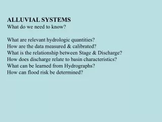
ALLUVIAL SYSTEMS What do we need to know? What are relevant hydrologic quantities? How are the data measured & calibrated? What is the relationship between Stage & Discharge? How does discharge relate to basin characteristics? What can be learned from Hydrographs?

E N D
ALLUVIAL SYSTEMS What do we need to know? What are relevant hydrologic quantities? How are the data measured & calibrated? What is the relationship between Stage & Discharge? How does discharge relate to basin characteristics? What can be learned from Hydrographs? How can flood risk be determined?
Quiz #4 at end 45 min Do any 4 problems, 25% each Name_____________ • 10. (10 points) This hydrograph, dated July 1996, is for the Selway River near Lowell, Idaho (USGS site # 13336500), which drains the uninhabited, mountainous, Bitterroot-Selway wilderness. In four sentences or less, describe and explain the variations you see, and determine anything you can about the character of this watershed. • 2. a. What is the “hydraulic radius” of a 90° V-Notch weir with water depth H? • b. Combine your result with the Chezy equation to determine a formula for the flow • rate Q of a v-notch weir for various water depths. If the level of the water doubles, • how much does the flow rate (discharge, Q) go up?
Need to know: Water Level = “Stage”, S Units: ft or meters Flow Rate = “Discharge”, Q Units ft3/s or m3/s and Variations with time: “Hydrograph” Meramec River, Missouri May 2000 S=27.8’ Q=56,000 cfs Criss
Hydrograph = plot of discharge vs. time, or = plot of stage vs. time Mean Flow Qmeanµ Area Flood Hydrographs Q µ Area small watersheds ? Q µ√(Area) large watersheds ? Storm & Annual Hydrographs can have rather similar forms
3788 mi2 = 9810 km2 Q, cfs calculated S, ft measured Ppt, in measured
175 mi2 = 453 km2 Q, cfs calculated S, ft measured Ppt, in measured
Stilling Well USGS Circ. 1123 Stage Measurement: Recording Stilling Well
Velocity Measurement Wading Rod <- Current Meter & Weight -> USGS
USGS Real-Time USGS Stream Gaging program (USGS Circular 1123) 7292 stations, 4200 telemetered GOES Geostationary Operations Environmental Satellite DOMSAT Domestic Satellite USES: Flood Forecasting Reservoir Operations Floodplain Engineering Flow Regulation Environmental & Pollution Regulation (Flow Minimums) Highway & Bridge Design Scientific Studies
USGS Real-Time Data Flow USGS Circular 1123
Eureka Gauging Station Since 1922 Criss
781 sq mi downstream 1475 sq mi downstream 3788 sq mi
S, ft. Q, cfs.
S, ft. Q, cfs.
S, ft. Q, cfs. + 0 cfs. -
259 sq. mi. 560 sq. mi.
199 sq. mi. downstream 781 sq. mi.
1475 sq mi downstream 3788 sq mi
Fetter, 2001 Freeze & Cherry, 1978 Criss 2003
Hydrograph = plot of discharge vs. time, or = plot of stage vs. time Mean Flow Qmeanµ Area Flood Hydrographs: dogma Q µ Area small watersheds ? Q µ√(Area) large watersheds ? Storm & Annual Hydrographs have rather similar forms
Hydrograph = plot of discharge vs. time, or = plot of stage vs. time Mean Flow Qmeanµ Area Flood Hydrographs: dogma Q µ Area small watersheds normal flow & floods Q µ√(Area) large watersheds record floods Storm & Annual Hydrographs have rather similar forms
STREAM GAGING:Establish link between Stage S & Discharge Q • THEORETICAL EQUATIONS • 2) SEMI-QUANTITATIVE EQUATIONS • 3) WEIRS • VELOCITY-AREA METHOD • THEORY of STEADY LAMINAR FLOW of Newtonian Fluid • Channel Flow (slot)u = (G/2m)(a2-y2) • uavg = Ga2/3m • Q ~g s W a3/3n cm3/sec • Pipe Flowu = (G/4m)(a2-r2) • uavg = Ga2/8m Q = g s p a4/8n cm3/sec • where G= “pressure gradient”, s=slope, 2a = slot depth or tube radius; W=width m viscosity; kinematic viscosity n =m/r cm2/sec
a 0 a a 0 a LAMINAR SLOT FLOW u =G(a2-y2)/2m uavg = Ga2/3m u =uavg @ a/√3 = 0.577 down LAMINAR PIPE FLOW u =G(a2-r2)/4m uavg = Ga2/8m u =uavg @ a/√2 = 0.707 down
LINEAR RESERVOIR (Chow, 14-27) Storage µ Outflow => S = Q/k Also, - dS/dt = Q(material balance requirement) Total flow = Base Flow: where Qo is (peak) discharge @ t 0 For complete depletion, the "Total Potential GW Discharge" is,
Qo=10 k=1
Note: not linear, but Concave Up
Q =7.07*Exp{-1.25*(t-tpk)} observed Q =1.2*Exp{-0.2083*(t-tpk)}
QBGS = 7.07* Q(0.35, 56.167, 1) observed observed
2) SEMI-QUANTITATIVE EQUATIONS a. Chezy Equn (1769)U = C Sqrt [RS] where “C” = discharge coeff.; “R” = hydraulic radius = A/P = cross sectional area/wetted perimeter “S” = energy gradient (slope of H2O sfc.) Units ? U vs Q ?
2) SEMI-QUANTITATIVE EQUATIONS a. Chezy Equn (1769)U = C Sqrt [RS] where “C” = discharge coeff., in units of √g. “R” = hydraulic radius = A/P = cross sectional area/wetted perimeter (in ft) “S” = energy gradient (slope of H2O sfc, dimensionless, e.g. ft/ft)
2) SEMI-QUANTITATIVE EQUATIONS a. Chezy Equn (1769)U = C Sqrt [RS] where “C” = discharge coeff., in units of √g. “R” = hydraulic radius = A/P = cross sectional area/wetted perimeter (in ft) “S” = energy gradient (slope of H2O sfc, dimensionless, e.g. ft/ft) b. Manning (1889) EqunUavg = Q/A = (1/n) R2/3 S1/2 m/s note: units! where: “n” = Manning roughness coeff. “n” , in units of sec/m1/3 n= 0.012 (concrete) n= 0.05 (rocky mountain stream) Note: 1) 1/n => 1.49/n if use ft, cfs (English units) 2) Manning eq is not compatible w/ Poiseuille flow as these have different proportionalities! 3) Manning Eq. is asserted to be the “same” as Chezy Equn! with n=3R1/6/2Cwhere C=Chezy coeff. impossible unless n or C depends on scale!
H 3) WEIRS Rectangular: Qcfs = 3.333 ( L - H/5) H3/2 90° V-Notch: Qcfs = 2.5 H5/2 where H, L in ft.Fetter p. 58 Culvert: See Chow 15-33; USGS Circ. 376) H
H 3) WEIRS Rectangular: Qm3/s = 1.84 ( L - H/5) H3/2 90° V-Notch: Qm3/s = 1.379 H5/2 where H, L in m.Fetter p. 58 Culvert: See Chow 15-33; USGS Circ. 376)
3) WEIRS Rectangular: Qm3/s = 1.84 ( L - H/5) H3/2 90° V-Notch: Qm3/s = 1.379 H5/2 where H, L in m.Fetter p. 58 “Note that equations…. are empirical and not subject to dimensional analysis”Fetter p. 58 Culvert: See Chow 15-33; USGS Circ. 376)
3) WEIRS Rectangular: Qcfs = 3.333 ( L - H/5) H3/2 90° V-Notch: Qcfs = 2.5 H5/2 Units! V-Notch: Cd= “discharge coeff”; Chow 7-46 Culvert: See Chow 15-33; USGS Circ. 376)
V-Notch Weir http://www.hubbardbrook.org
4) AREA-VELOCITY METHOD Current Meter Divide current into 15-30 segments Measure velocity @ 0.6*depth of segment (60% down) or, if channel is deep, take average v @ 0.8 and 0.2 times the depth. Q = Vavg*A Q = Sqi = Svidiwi where: vi= segment velocity di = segment depth wi = segment width Rating Curve: Graph of Discharge (cfs) vs. Stage (ft) Use entire river channel as a weir Need to revise curve if channel changes Qcfs = SaorQcfs = (S - So)awhereSo = stage @ zero flow Make polynomial fit USGS