Download
1 / 106
1.06k likes | 1.08k Vues
Develop algorithms to intercept illicit materials and weapons at U.S. ports with minimal cost, addressing false alarms and failed alarms. Explore sequential decision-making for container inspections using attributes like chemicals, cargo details, and imaging results.

E N D
Algorithms for Port of Entry Inspection: Finding Optimal Binary Decision Trees Fred S. Roberts Rutgers University
Port of Entry Inspection Algorithms • Goal: Find ways to intercept illicit • nuclear materials and weapons • destined for the U.S. via the • maritime transportation system • Goal: “inspect all containers arriving at ports” • Even carefully inspecting 8% of containers in Port of NY/NJ might bring international trade to a halt (Larrabbee 2002)
Aim: Develop decision support algorithms that will help us to “optimally” intercept illicit materials and weapons subject to limits on delays, manpower, and equipment • Find inspection schemes that minimize total “cost” including “cost” of false alarms (“false positives”) and failed alarms (“false negatives”) Port of Entry Inspection Algorithms Mobile Vacis: truck-mounted gamma ray imaging system
My work on port of entry inspection has gotten me and my students to some remarkable places. Port of Entry Inspection Algorithms Me on a Coast Guard boat in a tour of the harbor in Philadelphia Thanks to Capt. David Scott, Captain of Port, for taking us on the tour
Stream of containers arrives at a port • The Decision Maker’s Problem: • Which to inspect? • Which inspections next based on previous results? • Approach: • “decision logics” – Boolean methods • combinatorial optimization methods • Builds on ideas of Stroud and Saeger at Los Alamos National Laboratory • Need for new models and methods Sequential Decision Making Problem
Sequential Diagnosis Problem • Such sequential diagnosis problems arise in many areas: • Communication networks (testing connectivity, paging cellular customers, sequencing tasks, …) • Manufacturing (testing machines, fault diagnosis, routing customer service calls, …) • Medicine (diagnosing patients, sequencing treatments, …)
Containersarriving to be classified into categories. • Simple case: 0 = “ok”, 1 = “suspicious” • Inspection scheme: specifies which inspections are to be made based on previous observations Sequential Decision Making Problem
Sequential Decision Making ProblemFor Container Inspection • Containers have attributes, each • in a number of states • Sample attributes: • Levels of certain kinds of chemicals or biological materials • Whether or not there are items of a certain kind in the cargo list • Whether cargo was picked up in a certain port
Currently used attributes: • Does ship’s manifest set off an “alarm”? • What is the neutron or Gamma emission count? Is it above threshold? • Does a radiograph image come up positive? • Does an induced fission test come up positive? Sequential Decision Making Problem Gamma ray detector
We can imagine many other attributes • The project I have worked on is concerned with general algorithmic approaches. • We seek a methodology not tied to today’s technology. • Detectors are evolving quickly. Sequential Decision Making Problem
Simplest Case: Attributes are in state 0 or 1 (absent or present) • Then: Container is a bit string like 011001 • So: Classification is a decision functionF that assigns each bit string to a category. Sequential Decision Making Problem 011001 F(011001) If attributes 2, 3, and 6 are present, assign container to category F(011001).
If there are two categories, 0 and 1 (“safe” or “suspicious”), the decision function F is a Boolean function. • Example: • F(000) = F(111) = 1, F(abc) = 0 otherwise • This classifies a container as positive iff it has none of the attributes or all of them. Sequential Decision Making Problem 1 =
What if there are three categories, 0, ½, and 1?. • Example: • F(000) = 0, F(111) = 1, F(abc) = 1/2 otherwise • This classifies a container as positive if it has all of the attributes, negative if it has none of the attributes, and uncertain if it has some but not all of the attributes. • I won’t discuss this case. Sequential Decision Making Problem
Sequential Decision Making Problem • Given a container, test its attributes until know enough to calculate the value of F. • An inspection scheme tells us in which order to test the attributes to minimize cost. • Even this simplified problem is hard computationally.
This assumes F is known. • Simplifying assumption: Attributes are independent. • At any point we stop inspecting and output the value of F based on outcomes of inspections so far. • Complications: May be precedence relations in the components (e.g., can’t test attribute a4 before testing a6. • Or: cost may depend on attributes tested before. • F may depend on variables that cannot be directly tested or for which tests are too costly. Sequential Decision Making Problem
Such problems are hard computationally. • There are many possible Boolean functions F. • Even if F is fixed, problem of finding a good classification scheme (to be defined precisely below) is NP-complete. • Several classes of Boolean functions F allow for efficient inspection schemes: • - k-out-of-n systems • - Certain series-parallel systems • - Read-once systems • - “regular” systems • - Horn systems Sequential Decision Making Problem
n types of sensors measure presence or absence of the n attributes. • Many copies of each sensor. • Complication: different characteristics of sensors. • Entities come for inspection. • Which sensor of a given type to • use? • Think of inspection lanes and • waiting on line for inspection • Besides efficient inspection • schemes, could decrease costs by: • Buying more sensors • Change allocation of containers to sensor lanes. Sensors and Inspection Lanes
Sensors measure presence/absence of attributes: so 0 or 1 • Use two categories: 0, 1 (safe or suspicious) • Binary Decision Tree: • Nodes are sensors or categories • Two arcs exit from each sensor node, labeled left and right. • Take the right arc when sensor says the attribute is present, left arc otherwise Binary Decision Tree Approach
Reach category 1 from the root only through the path a0 to a1 to 1. • Container is classified in category 1 iff it has both attributes a0 and a1 . • Corresponding Boolean function: • F(11) = 1, F(10) = F(01) = F(00) = 0. Binary Decision Tree Approach Figure 1
Reach category 1 from the • root only through the path a1 • to a0 to 1. • Container is classified in category 1 iff it has both • attributes a0 and a1 . • Corresponding Boolean function: • F(11) = 1, F(10) = F(01) = F(00) = 0. • Note: Different tree, same function Binary Decision Tree Approach Figure 1
Reach category 1 from the • root only through the path a0 • to 1 or a0 to a1 to 1. • Container is classified in category 1 iff it has attribute • a0 or attribute a1 . • Corresponding Boolean function: • F(11) = 1, F(10) = F(01) = 1, F(00) = 0. Binary Decision Tree Approach Figure 1
Reach category 1 from • the root by: • a0 L to a1 R a2 R 1 or • a0 R a2 R 1 • Container classified in category 1 iff it has • a1 and a2 and not a0 or • a0 and a2 and possibly a1 . • Corresponding Boolean function: • F(111) = F(101) = F(011) = 1, F(abc) = 0 otherwise. Binary Decision Tree Approach Figure 2
This binary decision tree corresponds to the same Boolean function • F(111) = F(101) = F(011) = 1, F(abc) = 0 otherwise. • However,it has one less observation node ai. So, it is more efficient if all observations are equally costly and equally likely. Binary Decision Tree Approach Figure 3
So we have seen that a given Boolean function may correspond to different binary decision trees. • How do we find a low-cost or least-cost binary decision tree corresponding to a Boolean function? Binary Decision Tree Approach
Even if the Boolean function F is fixed, the problem of finding the “least cost” binary decision tree for it is very hard (NP-complete). • For small n = number of attributes, can try to solve it by trying all possible binary decision trees corresponding to the Boolean function F. • Even for n = 4, not practical. (n = 4 at Port of Long Beach-Los Angeles) Binary Decision Tree Approach Port of Long Beach
Promising Approaches: • Heuristic algorithms, approximations to optimal. • Special assumptions about the Boolean function F. • For “monotone” Boolean functions, integer programming formulations give promising heuristics. • Stroud and Saeger (Los Alamos • National Lab) enumerate all • “complete, monotone” Boolean functions • and calculate the least expensive • corresponding binary decision trees. • Their method practical for n up to 4, not n = 5. Binary Decision Tree Approach
Monotone Boolean Functions: • Given two bit strings x1x2…xn, y1y2…yn • Suppose that xi yi for all i implies that F(x1x2…xn) F(y1y2…yn). • Then we say that F is monotone. • Then 11…1 has highest probability of being in category 1. Binary Decision Tree Approach
Monotone Boolean Functions: • Given two bit strings x1x2…xn, y1y2…yn • Suppose that xi yi for all i implies that F(x1x2…xn) F(y1y2…yn). • Then we say that F is monotone. • Example: • n = 4, F(x) = 1 iff x has at least two 1’s. • F(1100) = F(0101) = F(1011) = 1, F(1000) = 0, etc. Binary Decision Tree Approach
Incomplete Boolean Functions: • Boolean function F is incomplete if F can be calculated by finding at most n-1 attributes and knowing the value of the input string on those attributes • Example: F(111) = F(110) = F(101) = F(100) = 1, F(000) = F(001) = F(010) = F(011) = 0. • F(abc) is determined without knowing b (or c). • F is incomplete. Binary Decision Tree Approach
Complete, Monotone Boolean Functions: • Stroud and Saeger: algorithm for enumerating binary decision trees implementing complete, monotone Boolean functions. • Feasible to implement up to n = 4. • Then you can find least cost tree by enumerating all binary decision trees corresponding to a given complete, monotone Boolean function and repeating this for all complete, monotone Boolean functions. Binary Decision Tree Approach
Complete, Monotone Boolean Functions: • Stroud and Saeger: algorithm for enumerating binary decision trees implementing complete, monotone Boolean functions. • n = 2: • There are 6 monotone Boolean functions. • Only 2 of them are complete, monotone • There are 4 binary decision trees for calculating these 2 complete, monotone Boolean functions. Binary Decision Tree Approach
Complete, Monotone Boolean Functions: • n = 3: • 9 complete, monotone Boolean functions. • 60 distinct binary trees for calculating them Binary Decision Tree Approach
Complete, Monotone Boolean Functions: • n = 4: • 114 complete, monotone Boolean functions. • 11,808 distinct binary decision trees for calculating them. • (Compare 1,079,779,602 BDTs for all Boolean functions) Binary Decision Tree Approach
Complete, Monotone Boolean Functions: • n = 5: • 6894 complete, monotone Boolean functions • 263,515,920 corresponding binary decision trees. • Combinatorial explosion! • Need alternative approaches; enumeration not feasible! • (Even worse: compare 5 x 10¹⁸ BDTs corresponding to all Boolean functions) Binary Decision Tree Approach
Cost Functions • So far, we have figured one binary decision tree is cheaper than another if it has fewer nodes. • This is oversimplified. • There are more complex costs involved than number of sensors in a tree.
Cost Functions • Stroud-Saeger method applies to more sophisticated cost models, not just cost = number of sensors in the BDT. • Using a sensor has a cost: • Unit cost of inspecting one item with it • Fixed cost of purchasing and deploying it • Delay cost from queuing up at the sensor station • Preliminary problem: disregard fixed and delay costs. Minimize unit costs.
Tradeoff between fixed costs and delay costs: Add more sensors cuts down on delays. • More sophisticated models describe the process of containers arriving • There are differing delay times for inspections • Use “queuing theory” to find average delay times under different models Cost Functions: Delay Costs
Cost Functions • Unit Cost Complication: How many nodes of the decision tree are actually visited during average container’s inspection? Depends on “distribution” of containers. • Answer can also depend on probability of sensor errors and probability of “bomb” in a container.
Cost Functions:Unit CostsTree Utilization • In our early models, we assume we are given probability of sensor errors and probability of bomb in a container. • This allows us to calculate “expected” cost of utilization of the tree Cutil.
Cost Functions • OTHER COSTS: • Cost of false positive: Cost of additional tests. • If it means opening the container, it’s expensive. • Cost of false negative: • Complex issue. • What is cost of a bomb going off in Manhattan?
One Approach to False Positives/Negatives: • Assume there can be Sensor Errors • Simplest model: assume that all sensors checking for attribute ai have same fixed probability of saying ai is 0 if in fact it is 1, and similarly saying it is 1 if in fact it is 0. • More sophisticated analysis later describes a model for determining probabilities of sensor errors. • Notation: X = state of nature (bomb or no bomb) • Y = outcome (of sensor or entire inspection process). Cost Functions: Sensor Errors
A A B 0 B 0 C 1 C 1 1 0 1 0 Probability of Error for The Entire Tree State of nature is one (X = 1), presence of a bomb State of nature is zero (X = 0), absence of a bomb Probability of false positive (P(Y=1|X=0)) for this tree is given by Probability of false negative (P(Y=0|X=1)) for this tree is given by P(Y=1|X=0) = P(YA=1|X=0) * P(YB=1|X=0) + P(YA=1|X=0) *P(YB=0|X=0)* P(YC=1|X=0) Pfalsepositive P(Y=0|X=1) = P(YA=0|X=1) + P(YA=1|X=1) *P(YB=0|X=1)*P(YC=0|X=1) Pfalsenegative
Cost Function used for Evaluating the Decision Trees. CTot =CFalsePositive *PFalsePositive + CFalseNegative *PFalseNegative+ Cutil CFalsePositive is the cost of false positive (Type I error) CFalseNegative is the cost of false negative (Type II error) PFalsePositive is the probability of a false positive occurring PFalseNegative is the probability of a false negative occurring Cutil is the expected cost of utilization of the tree.
Cost Function used for Evaluating the Decision Trees. CFalsePositive is the cost of false positive (Type I error) CFalseNegative is the cost of false negative (Type II error) PFalsePositive is the probability of a false positive occurring PFalseNegative is the probability of a false negative occurring Cutil is the expected cost of utilization of the tree. PFalsePositive and PFalseNegative are calculated from the tree. Cutil is calculated from tree and probabilities of bomb in container and probability of sensor errors. CFalsePositive, CFalseNegative are input – given information.
Stroud Saeger Experiments • Stroud-Saeger ranked all trees formed from 3 or 4 sensors A, B, C and D according to increasing tree costs. • Used cost function defined above. • Values used in their experiments: • CA = .25; P(YA=1|X=1) = .90; P(YA=1|X=0) = .10; • CB = 10; P(YC=1|X=1) = .99; P(YB=1|X=0) = .01; • CC = 30; P(YD=1|X=1) = .999; P(YC=1|X=0) = .001; • CD = 1; P(YD=1|X=1) = .95; P(YD=1|X=0) = .05; • Here, Ci = unit cost of utilization of sensor i. • Also fixed were: CFalseNegative, CFalsePositive, P(X=1)
Sensitivity Analysis • When parameters in a model are not known exactly, the results of a mathematical analysis can change depending on the values of the parameters. • It is important to do a sensitivity analysis: let the parameter values vary and see if the results change. • So, do the least cost trees change if we change values like probability of a bomb, cost of a false positive, etc?
Stroud Saeger Experiments: Our Sensitivity Analysis • We have explored sensitivity of the Stroud-Saeger conclusions to variations in values of the three parameters: CFalseNegative, CFalsePositive, P(X=1) • Extensive computer experimentation. • Fascinating results. • To start, we estimated high and low values for the parameters.
Stroud Saeger Experiments: Our Sensitivity Analysis • CFalseNegativewas varied between 25 million and 10 billion dollars • Low and high estimates of direct and indirect costs incurred due to a false negative. • CFalsePositive was varied between $180 and $720 • Cost incurred due to false positive (4 men * (3 -6 hrs) * (15 – 30 $/hr) • P(X=1)was varied between 1/10,000,000 and 1/100,000
Stroud Saeger Experiments: Our Sensitivity Analysis n = 3 (use sensors A, B, C) • Varied the parameters CFalseNegative, CFalsePositive, P(X=1) • We chose the value of one of these parameters from the interval of values • Then explored the highest ranked tree as the other two parameters were chosen at random in the interval of values. • 10,000 experiments for each fixed value. • We looked for the variation in the top-ranked tree and how the top-rank related to choice of parameter values. • Very surprising results.
Frequency of Top-ranked Trees when CFalseNegative and CFalsePositive are Varied • 10,000 randomized experiments (randomly selected values of CFalseNegative and CFalsePositive from the specified range of values) for the median value of P(X=1). • The above graph has frequency counts of the number of experiments when a particular tree was ranked first or second or third and so on. • Only three trees (7, 55 and 1) ever came first. 6 trees came second, 10 came third, 13 came fourth.