Binary search trees
Binary search trees. Definition Binary search trees and dynamic set operations Balanced binary search trees Tree rotations Red-black trees Move to front “balancing” technique Unsorted linked lists Splay trees. Binary search trees. Basic tree property For any node x

Binary search trees
E N D
Presentation Transcript
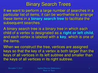
Binary search trees • Definition • Binary search trees and dynamic set operations • Balanced binary search trees • Tree rotations • Red-black trees • Move to front “balancing” technique • Unsorted linked lists • Splay trees
Binary search trees • Basic tree property • For any node x • left subtree has nodes ≤x • right subtree has nodes ≥ x
BSTs and Dynamic Sets • Dynamic set operations and binary search trees • Search(S,k) • Insert(S,x) • Delete(S,x) • Minimum or Maximum(S) • Successor or Predecessor (S,x) • List All(S) • Merge(S1,S2)
Dynamic Set Operations • Listall(T)? • time to list? • Search(T,k)? • search time? • Minimum(T)? Maximum(T)? • search time? • Successor(T,x)? Predecessor(T,x)? • Search time • Simple Insertion(T,x)
Simple deletion • Delete(T,x): Three possible cases: • a) x is a leaf : • b) x has one child : • c) x has two children : Replace x with successor(x). • Successor(x) has at most one child (why?); • Use step a or b on successor(x)
Simple binary search trees • What is the expected height of a binary search tree? • Difficult to compute if we allow both insertions and deletions • With insertions, analysis of section 12.4 shows that expected height is O(log n) • Implications about BSTs as dynamic sets?
Tree-Balancing Algorithms • Tree rotations • Red-Black Trees • Splay Trees • Others • AVL Trees • 2-3 Trees and 2-3-4 Trees
Tree Rotations Right Rotate(T,A) A B T1 B A T3 T1 T2 Left Rotate(T,B) T2 T3
Red-Black Trees • All nodes in the tree are either red or black. • Every null-child is included and colored black. • All red nodes must have two black children. • Every path from any node x (including the root) to a leaf must have the same number of black nodes. • How balanced of a tree will this produce? • How hard will it be to maintain?
Insertion(T,z) • Find place to insert using simple insertion • Color node z as red • Fix up tree so that it is still a red-black tree • What needs to be fixed? • Problem 1: z is root (first node inserted) • Minor detail • Problem 2: parent(z) is red
z z RB-Insert-Fixup • Situation: parent(z) is red and z is red • Case 1: uncle(z) is red • Then make both uncle(z) and parent(z) black and p(p(z)) red and recurse up tree
B A T1 A z B z T3 T2 T3 T1 T2 RB-Insert-Fixup(parent(z) is right child of parent(parent(z))) • Situation: parent(z) is red and z is red • Case 2: uncle(z) is black and z is a left child • Right rotate to make into case 3
C B B C A T1 A z T1 T2 T3 T2 T3 RB-Insert-Fixup(parent(z) is right child of parent(parent(z))) • Situation: parent(z) is red and z is red • Case 3: uncle(z) is black and z is a left child • Left rotate to make B root of tree
RB-Insert-Fixup Analysis(parent(z) is right child of parent(parent(z))) • Situation: parent(z) is red and z is red • Case 1: no rotations, always moving up tree • Cases 2 and 3: At most 2 rotations total and tree ends up balanced • No more need to fix up once these cases are met • Total cost: at most 2 rotations and log n operations
Delete(T,z) • Find node y to delete using simple deletion • Let x be a child of y if such a child exists (otherwise x is a null child) • If y is black, fix up tree so that it is still a red-black tree • What needs to be fixed? • Problem 1: y was root, so now we might have red root • Problem 2: x and parent(y) are both red • Problem 3: Removal of y violates black height properties of paths that used to go through y
Move To Front (MTF) Technique • A powerful “balancing” mechanism is the “move to front” idea • This technique is effective in managing both unsorted lists and binary search trees • The idea: Whenever an item is accessed (by search or by insertion), it is always moved to the front • In a list, the front is well-defined • In a binary search tree, the front of the tree is the root • A tree that implements this idea is called a splay tree • Rotations are not simple single rotations but occur in pairs • We give some intuition about the power of MTF
Effectiveness in lists • Reference: Amortized efficiency of list update and paging rules, Sleator and Tarjan, CACM 1985 • Problem statement: • Suppose you are maintaining an unsorted list where every search must progress from the front of the list to the item (or end of list if search is unsuccessful) • Operations: search, insert, delete • Costs: finding or deleting the ith item costs i • Inserting a new item costs n+1 • Immediately after an insertion or search of an item i, item i may be moved anywhere closer to the front of the list at no extra cost • Goal: Find a way to manage list that minimizes total cost of a sequence of operations
Notation for computing costs • S: sequence of requests • (insertions, deletions, searches) • A: any algorithm for maintaining list • including those those that know S in advance • cA(S): cost incurred by algorithm A on sequence S not including paid exchanges • xA(S): # of paid exchanges for A on S • fA(S): # of free exchanges for A on S • Example: • List: 5, 9, 2, 7, 3, 6 and we search for 7 • MTF then has list with 7, 5, 9, 2, 3, 6 • cMTF(S) increases by 4 • xMTF(S) increases by 0 since moving 7 to the front is a free • fMTF(S) increases by 3 since we made 3 free exchanges to move 7
Performance of MTF • Thm: For any algorithm A and any sequence S xMTF(S) + cMTF(S) ≤ 2cA(S)+ xA(S) – FA(S) – m • Observation: xMTF(S) = 0 • Interpretation • MTF incurs at most twice the cost of any other algorithm, even those that know the request sequence in advance
Direct Cost Comparison • The ideal approach to proving this result is that for each operation, MTF incurs a cost that is at most twice that of algorithm A • However, this is clearly not always true • Example just before tth operation search(1): • A’s list: 1, 20, 7, 9, 3, 5, 24, 4, 8 • A’s cost is just 1 • MTF’s list: 5, 24, 8, 3, 9, 7, 20, 4, 1 • MTF’s cost is 9 • How can this happen? • Well, since last access to item 1, items 5, 24, 8, 3, 9, 7, 20 and 4 have been accessed. • Thus, A must have done some extra work since last access to 1 in order to have 1 at the current front of the list • This leads to ideas of potential function and amortized analysis
Potential Function Φ • Consider A, MTF, and S • Let t be the number of operations performed so far (0 ≤ t ≤ |S|) • For any t, we define Φ(t) to be the number of inversions between A’s list and MTF’s list • Inversion: a pair of elements x,y s.t. x appears before y in one list and y appears before x in the other list • Example • MTF: 1, 7, 2, 5 • A: 2, 1, 5, 7 • Inversions: (1,2), (2,7), (5,7)
Amortized Cost • Cost cA(t) is the cost of the tth operation for algorithm A • Amortized cost aA(t) of the tth operation is cA(t) + Φ(t) - Φ(t-1) • Cost of tth operation + change in potential fct • Key observation Σt aMTF(t) = Σt cMTF(t) + Φ(t) - Φ(t-1) = Φ(|S|) - Φ(0) + Σt cMTF(t) Thus, cMTF(S) = Σt cMTF(t) = Φ(0) - Φ(|S|) + Σt aMTF(t) Thus, cMTF(S) ≤ Σt aMTF(t) • Note Φ(0) = 0 and Φ(|S|) ≥ 0
Amortized Cost Comparison • Our revised goal is to show that MTF incurs an amortized cost that is at most twice that of algorithm A • Example just before tth operation search(1): • A’s list: 1, 20, 7, 9, 3, 5, 24, 4, 8 • A’s cost is just 1 • MTF’s list: 5, 24, 8, 3, 9, 7, 20, 4, 1 • MTF’s list afterwards: 1, 5, 24, 8, 3, 9, 7, 20, 4, 1 • MTF’s direct cost is 9 • The change in potential function is -8 as 8 inversions (all involving 1) are eliminated after 1 is moved to the front of the list • MTF’s amortized cost is 1
Amortized Cost Comparison Cont’d • General case • We are searching for x which is at position i in A’s list and k in MTF’s list • Direct costs • A’s cost to access x is then i • MTF’s cost to access x is k • Potential function changes • Let y be the number of items that precede x in MTF’s list but follow x in A’s list • This means k-y-1 items precede x in both lists • Note k-y ≤ i. Why? • After x is moved to front of MTF’s list • y inversions are eliminated • k-y-1 inversions are created • Thus potential function change is k-2y-1 • MTF’s amortized cost is thus: k + (k-2y-1) = 2(k-y) -1 ≤ 2i-1 • Similar analysis holds for other operations
Splay Tree Performance • Analysis of splay trees also uses a potential function and amortized analysis • Individual operations may take O(n) time • However, it can be shown that any sequence of m operations including n insertions starting with an empty tree take O(m log n) time • Static optimality theorem • For any sequence of access operations, a splay tree is asymptotically as efficient as the optimum static search tree (that cannot perform any rotations)
Dynamic Optimality Conjecture • Splay trees are as asymptotically fast on any sequence of operations as any other type of search tree with rotations. • What does this mean? • Worst case sequence of splay tree operations takes amortized O(log n) time per operation • Some sequences of operations take less. • Accessing the same ten items over and over again • Splay tree should then take less on these sequences as well. • One special case that has been proven: • search in order from the smallest key to the largest key • the total time for all n operations is O(n)