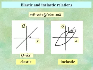
Elastic and inelastic relations
490 likes | 616 Vues
Learn about energy dissipation, hysteretic damping, Newmark's design criteria, ductility factor, and structural strength in dynamic systems. Understand the principles behind calculations and criteria for optimal performance.

Elastic and inelastic relations
E N D
Presentation Transcript
Elastic and inelastic relations .. . ..mx+cx+Q(x)= -ma Q Q x x Q=kx elastic inelastic
Exercise 1 (A hysteretic energy dissipation index Eh) A hysteretic energy dissipation index Eh corresponds to equivalent viscous damping factor h. Derive the equation (3.1) by calculating energy dissipation ΔU by viscous damping per cycle under the ‘resonant steady-state’ and putting ΔU = ΔW. Eh = ΔW/2πFmDm(3.1) c: damping coefficient(=2hm ), m: mass of the system : natural circular frequency(= ) k=Fm/Dmy: amplitude, a:maximum amplitude(=Dm)p:input frequency,: phase difference‘Resonant steady-state’ means p= .
Example 2 (A hysteretic energy dissipation index Eh in the case of elasto-plastic model) Derive the equation shown below by calculating energy dissipation ΔW under the ‘resonant steady-state’ in the case of elasto-plastic model.
Excercise 2 (A hysteretic energy dissipation index Eh in the case of Clough model) Derive the equation (3.8) by calculating energy dissipation ΔW under the ‘resonant steady-state’ in the case of modified Clough model. (3.8)
Simple method to get elastic period of SDOF system w: a unit weight(=12000N/m2), ΣAf: sum of whole floor area of the building(m2) ,g: gravity(cm/s2), Fc: compressive strength of concrete (N/mm2) , b: width of a column(cm), D: depth of a olumn(cm), h: story height(cm), n: number of story moment of inertia of a column (cm4) stiffness of concrete (N/mm2)
Simple method to get base shear coefficient of SDOF system τc: ultimate shear strength of columns(N/mm2=Fc/15), Ac: sum of 1st story column section area(cm2) , w: a unit weight(=12000N/m2), ΣAf: sum of whole floor area of the building(m2)
Example 3 (Simple method to get fundamental parameters of SDOF system ) story height: 3.6m plan elevation ⇔longitudinal direction 3-story building:column size: 60cm x 60cmFc= 24(N/mm2)
Exercise 3 (Simple method to get fundamental parameters of SDOF system ) story height: 3.5m plan elevation ⇔longitudinal direction 12-story building:column size: 95cm x 95cmFc= 48(N/mm2)
Newmark’s design criteria Newmark’s design criteria was used to decide strength of the system for each input strong ground motion. ・property of energy conservation: For short period systems (T<0.5s) the energy dissipation is constant. ・property of displacement conservation: For long period systems (T>0.5s) the response displacement is constant.
Property of energy conservation For short period systems (T<0.5s)The area of trapezoid OBCE= the one of △OAD (μδy+(μ-1) δy)Qy/2=δL*QL/2 δy =Qy/k, δL =QL/k
Property of displacement conservation For long period systems (T>0.5s)inelastic response displacement is the same as elastic response displacement. μδy= QL/k δy =Qy/k
Example 5 (Newmark’s design criteria) Calculate response displacement in the case that 1) elastic period=0.3 sec., base shear coefficient= 0.4,elastic response acceleration=0.8g at 0.3 sec.2) elastic period=1.0 sec., base shear coefficient= 0.1,elastic response acceleration=0.2g at 1.0 sec.
Exercise 5 (Newmark’s design criteria) Calculate response displacement under the input of El-Centro NSusing elastic spectra (damping factor=0.05, Fig.4.3,(b), p.139) and Newmark’s design criteria in the case that 1) 7-story reinforced concrete building (base shear coefficient= 0.3, story height=2.8(m))2) 20-story steel building (base shear coefficient= 0.05, story height=3.5(m)) T=0.02H (T: period of the building (s), H: height of the building(m)) for reinforced concrete buildingT=0.03H (T: period of the building (s), H: height of the building(m)) for steel building
Tripartite response spectra Response spectra which show response acceleration, velocity and displacement simultaneouslyusing the relations:SV=ωSDSA=ωSV=ω2SDSD: response displacementSV: response pseudo-velocity SA: response pseudo-acceleration
Ductility factor Ductility factor is used as the index of representing the damage level. Ductility factor μ is defined as the ratio of the maximum response displacement x to the yielding displacement xy.
Ductility factor of short and long period system Short period system long period system μ=dm/dy=5 μ=dm/dy=2
Response ductility factor spectra Ductility factors were calculated in the case of bilinear Takeda model under the input of El-Centro NS and Fukiai (Kobe EQ.) changing the base shear coefficient.
Response ductility factor spectra Input: El-Centro NS Bilinear Takeda model
Response ductility factor spectra Input: Fukiai (Kobe EQ.) Bilinear Takeda model
Comparison of response ductility factor spectra Input: El-Centro NS Bilinear Takeda model Input: Fukiai (Kobe EQ.) Bilinear Takeda model
Required strength Required strength which give maximum response ductility factors within constant values is important, because we need design base shear coefficient in the structural design. ↑ Allowable ductility factor μa
Required strength spectra Input: El-Centro NS Bilinear Takeda model
Required strength spectra Input: Fukiai (Kobe EQ.) Bilinear Takeda model
Comparison of required strength spectra Input: El-Centro NS Bilinear Takeda model Input: Fukiai (Kobe EQ.) Bilinear Takeda model
Example 8 (Calculation of required strength spectrum from response ductility factor spectra) Calculate required strength (base shear coefficient) spectrum from response ductility factor spectra in the case that allowable ductility factor=4, model: bilinear Takeda model (α=0.5, β=0.01)under the input of El-Centro NS. Response ductility factor spectra changing base shear coefficient of the system input motion: El-Centro NS T(s) Cy=0.005 0.01 0.02 0.05 0.1 0.2 0.3 0.4 0.5 0.100 99.999 99.999 99.999 99.999 99.999 38.270 8.309 1.826 1.174 0.200 99.999 99.999 99.999 99.999 65.070 19.300 6.894 2.350 1.557 0.500 99.999 99.999 99.999 45.490 13.500 6.573 3.564 2.734 1.987 1.000 99.999 73.020 24.880 13.080 4.469 2.071 1.474 1.285 1.030 1.500 74.490 33.440 13.380 5.099 1.954 0.947 0.632 0.474 0.379 2.000 47.700 21.080 7.728 3.817 1.831 0.887 0.592 0.444 0.355 3.000 21.190 9.574 3.388 1.865 1.114 0.570 0.380 0.285 0.228 99.999: greater than 100
Example 8 (Calculation of required strength spectrum from response ductility factor spectra) Calculate required strength (base shear coefficient) spectrum from response ductility factor spectra in the case that allowable ductility factor=4, model: bilinear Takeda model (α=0.5, β=0.01)under the input of El-Centro NS. Response ductility factor spectra changing base shear coefficient of the system input motion: El-Centro NS T(s) Cy=0.005 0.01 0.02 0.05 0.1 0.2 0.3 0.4 0.5 0.100 99.999 99.999 99.999 99.999 99.999 38.270 8.309 1.826 1.174 0.200 99.999 99.999 99.999 99.999 65.070 19.300 6.894 2.350 1.557 0.500 99.999 99.999 99.999 45.490 13.500 6.573 3.564 2.734 1.987 1.000 99.999 73.020 24.880 13.080 4.469 2.071 1.474 1.285 1.030 1.500 74.490 33.440 13.380 5.099 1.954 0.947 0.632 0.474 0.379 2.000 47.700 21.080 7.728 3.817 1.831 0.887 0.592 0.444 0.355 3.000 21.190 9.574 3.388 1.865 1.114 0.570 0.380 0.285 0.228 99.999: greater than 100
Required strength spectrum (allowable ductility factor=4 ) by El-Centro NS requiredT(s) strength (base shear coefficient) 0.1 0.366 0.2 0.364 0.5 0.286 1.0 0.120 1.5 0.067 2.0 0.049 3.0 0.019
Exercise 8 (Calculation of required strength spectrum from response ductility factor spectra) Calculate required strength (base shear coefficient) spectrum from response ductility factor spectra in the case that allowable ductility factor=4, model: bilinear Takeda model (α=0.5, β=0.01)under the input of Taft EW and compare it with El-Centro NS. Response ductility factor spectra changing base shear coefficient of the system input motion: Taft EW T(s) Cy=0.005 0.01 0.02 0.05 0.1 0.2 0.3 0.4 0.5 0.100 99.999 99.999 99.999 99.999 84.430 1.109 0.720 0.540 0.432 0.200 99.999 99.999 99.999 74.450 23.240 4.561 1.577 1.079 0.859 0.500 99.999 99.999 32.930 13.910 5.297 1.396 1.168 0.864 0.691 1.000 91.840 37.000 10.040 3.978 1.734 0.793 0.529 0.396 0.317 1.500 51.110 18.410 7.052 2.825 1.389 0.655 0.437 0.327 0.262 2.000 31.780 11.420 4.222 1.352 0.855 0.428 0.285 0.214 0.171 3.000 15.710 6.619 2.097 0.957 0.479 0.239 0.160 0.120 0.096 99.999: greater than 100
Exercise 8 (Calculation of required strength spectrum from response ductility factor spectra) Calculate required strength (base shear coefficient) spectrum from response ductility factor spectra in the case that allowable ductility factor=4, model: bilinear Takeda model (α=0.5, β=0.01)under the input of Taft EW and compare it with El-Centro NS. Response ductility factor spectra changing base shear coefficient of the system input motion: Taft EW T(s) Cy=0.005 0.01 0.02 0.05 0.1 0.2 0.3 0.4 0.5 0.100 99.999 99.999 99.999 99.999 84.430 1.109 0.720 0.540 0.432 0.200 99.999 99.999 99.999 74.450 23.240 4.561 1.577 1.079 0.859 0.500 99.999 99.999 32.930 13.910 5.297 1.396 1.168 0.864 0.691 1.000 91.840 37.000 10.040 3.978 1.734 0.793 0.529 0.396 0.317 1.500 51.110 18.410 7.052 2.825 1.389 0.655 0.437 0.327 0.262 2.000 31.780 11.420 4.222 1.352 0.855 0.428 0.285 0.214 0.171 3.000 15.710 6.619 2.097 0.957 0.479 0.239 0.160 0.120 0.096 99.999: greater than 100
Required strength spectra (allowable ductility factor=4 ) by El-Centro NS and Taft EW required strength (base shearT(s) coefficient) El-Centro Taft NS EW 0.1 0.366 0.197 0.2 0.364 0.219 0.5 0.286 0.133 1.0 0.120 0.050 1.5 0.067 0.042 2.0 0.049 0.022 3.0 0.019 0.016
Equivalent linear system Inelastic responses can be estimated by equivalent linear systems with equivalent period and equivalent viscous damping. equivalent period Q Q x x with equivalent viscous damping inelastic elastic
Method to calculate inelastic responses by equivalent linear systems How to decide equivalent period and damping equivalent period: period corresponding maximum displacement equivalent damping: equivalent viscous damping
Example 9 (Required strength spectrum by equivalent linear system) Calculate required strength (base shear coefficient) spectrum(T=0.1, 0.2, 0.5, 1.0, 1.5, 2.0 and 3.0 s)by equivalent linear system in the case that allowable ductility factor=4, model: bilinear Takeda model (α=0.5, β=0.01)under the input of El-Centro NSfrom elastic response spectra (h=0.05)→using the damping reduction factor inEquation shown below andcompare it with required strength spectrum by inelastic systemand Newmark’s design criteria. responseT(s) acceleration (cm/s2)0.1 560.70.2 640.70.3 695.9 0.4 601.80.5 820.5 1.0 507.41.5 186.7 2.0 174.9 3.0 112.3 4.0 45.4 6.0 31.0 Fh: reduction factor from h=0.05, h: damping factor
Required strength spectrum (allowable ductility factor=4 ) by El-Centro NS using equivalent linear system comparing with actual spectrum Required strength (base shear coefficient) Inelastic Equivalent Newmark’s T(s) system linear design system criteria 0.1 0.366 0.386 0.216 0.2 0.364 0.363 0.217 0.5 0.286 0.306 0.316, 0.209 1.0 0.120 0.105 0.129 1.5 0.067 0.068 0.048 2.0 0.049 0.027 0.045 3.0 0.019 0.019 0.029
Required strength spectrum (allowable ductility factor=4 ) by El-Centro NS using equivalent linear system comparing with actual spectrum Required strength (base shear coefficient) Inelastic EquivalentT(s) system linear system 0.1 0.366 0.386 0.2 0.364 0.363 0.5 0.286 0.306 1.0 0.120 0.105 1.5 0.067 0.068 2.0 0.049 0.027 3.0 0.019 0.019
Exercise 9 (Required strength spectrum by equivalent linear system) Calculate required strength (base shear coefficient) spectrum(T=0.1, 0.2, 0.5, 1.0, 1.5, 2.0 and 3.0 s)by equivalent linear system in the case that allowable ductility factor=4, model: bilinear Takeda model (α=0.5, β=0.01)under the input of Taft EWfrom elastic response spectra (h=0.05)→using the damping reduction factor inEquation shown below andcompare it with required strength spectrum by inelastic systemand Newmark’s design criteria. responseT(s) acceleration (cm/s2)0.1 211.90.2 422.50.3 398.40.4 387.40.5 340.31.0 156.41.5 129.32.0 84.93.0 47.24.0 27.16.0 22.7 Fh: reduction factor from h=0.05, h: damping factor
Required strength spectrum (allowable ductility factor=4 ) by Taft EW using equivalent linear system comparing with actual spectrum Required strength (base shear coefficient) Inelastic EquivalentT(s) system linear system 0.1 0.197 0.255 0.2 0.219 0.233 0.5 0.133 0.094 1.0 0.050 0.051 1.5 0.042 0.028 2.0 0.022 0.016 3.0 0.016 0.014
Required strength spectrum (allowable ductility factor=4 ) by Taft EW using equivalent linear system comparing with actual spectrum Required strength (base shear coefficient) Inelastic Equivalent Newmark’s T(s) system linear design system criteria 0.1 0.197 0.255 0.082 0.2 0.219 0.233 0.163 0.5 0.133 0.094 0.131, 0.087 1.0 0.050 0.051 0.040 1.5 0.042 0.028 0.033 2.0 0.022 0.016 0.022 3.0 0.016 0.014 0.012
Example & Excersise10 (Prediction of response ductility factor from elastic response using equivalent linear system and comparison with actual structural damage) Calculate response ductility factor in the case of longitudinal direction of Kuoshing National Elementary School Building B under the input of recorded strong ground motion of 1999 Chi-chi, Taiwan earthquake using equivalent linear system and compare with actual structural damage.
Elastic response spectrum at Shikang National Elementary School Building A
Elastic response spectrum at Kuoshing National Elementary School Building B
Information of the buildings Shikang Kuoshing N.E.S. N.E.S. Building A Building B unit of weight 1.2 1.2 tonf/m2 Fc 154.7 216.5 kgf/cm2 No. of story 3 3 span length (longitudinal) column1 depth(longitudinal) 33.0 50.0 cm column1 depth(transvers) 46.8 58.0 cm transvers column1 column2 depth(longitudinal) 52.3 50.0 cm column2 depth(transvers) 52.4 58.0 cm span length1 column3 depth(longitudinal) 40.0 50.0 cm (transvers) column3 depth(transvers) 65.0 58.0 cm column2 span length1(transvers) 783.2 500.0 cm span length2(transvers) 261.3 cm span length2 (transvers) span l ength(longitudinal) 300.0 400.0 cm column3 story height 343.0 360.0 cm No. of span(longitudinal) 16 5 No. of span(transvers) 2 5 longitudinal
Simple method to get elastic period of SDOF system w: a unit weight(=12000N/m2), ΣAf: sum of whole floor area of the building(m2) ,g: gravity(cm/s2), Fc: compressive strength of concrete (N/mm2) , b: width of a column(cm), D: depth of a olumn(cm), h: story height(cm), n: number of story moment of inertia of a column (cm4) stiffness of concrete (N/mm2)
Simple method to get base shear coefficient of SDOF system τc: ultimate shear strength of columns(N/mm2=Fc/15), Ac: sum of 1st story column section area(cm2) , w: a unit weight(=12000N/m2), ΣAf: sum of whole floor area of the building(m2)
Equivalent viscous damping and damping reduction factor Decide μso that response acceleration is equal to base shear coefficient at equivalent period T’ and equivalent viscous damping factor Eh from elastic response spectrum of damping factor 0.05.