Download
1 / 12
120 likes | 146 Vues
Learn how to analyze motion data, calculate instantaneous velocity, and choose accurate time intervals for precise calculations in physics using calculus. Understand the significance of change and calculus in studying moving objects.

E N D
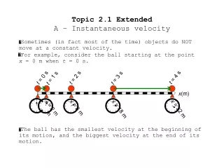
x(m) Topic 2.1 ExtendedA – Instantaneous velocity Sometimes (in fact most of the time) objects do NOT move at a constant velocity. For example, consider the ball starting at the point x = 0 m when t = 0 s. t = 4 s t = 0 s t = 2 s t = 3 s t = 1 s x = 8 m x = 2 m x = 0 m x = 32 m x = 18 m The ball has the smallest velocity at the beginning of its motion, and the biggest velocity at the end of its motion.
x(m) Topic 2.1 ExtendedA – Instantaneous velocity t = 4 s t = 0 s t = 2 s t = 3 s t = 1 s x = 8 m x = 2 m x = 0 m x = 32 m x = 18 m To get a handle on its motion, we graph the data. t(s) x(m) 0 0 1 2 2 8 3 18 4 32 We begin by making a table of values.
t(s) x(m) 0 0 1 2 2 8 3 18 4 32 Topic 2.1 ExtendedA – Instantaneous velocity Then we plot the data on a suitable coordinate system: 32 18 x(m) 8 2 0 t(s) 4 3 0 2 1
32 18 x(m) 8 V0.5 V2.5 2 0 t(s) 4 3 0 2 1 Topic 2.1 ExtendedA – Instantaneous velocity Note that the average velocity now depends on WHICH TWO POINTS WE CHOOSE: Which slope is the best estimate for the velocity at t = 0.5 seconds? Which slope is the best estimate for the velocity at t = 2.5 seconds? FYI: The closer together the two points on the graph are, the better the estimate of the velocity of the particle BETWEEN THE TWO POINTS.
32 Average Velocity v = 18 Instantaneous Velocity x(m) 8 2 0 t(s) 4 3 0 2 1 FYI: In words, the instantaneous velocity is the velocity of the MOMENT, not some sort of average. FYI: The key is to choose your times VERY CLOSE TOGETHER to get the most exact value for v. Topic 2.1 ExtendedA – Instantaneous velocity Recall that the average velocity was given by FYI: That is the meaning of t→0. x t We now define the instantaneous velocityv like this: x t limit t→0 v = The above is read "vee equals the limit, as delta tee approaches zero, of delta ex over delta tee."
32 18 x(m) 8 2 0 t(s) 4 3 0 2 1 FYI: All branches of the so-called "hard" sciences use calculus. The fields of engineering, statistical analysis, computer science, and even political science, use calculus. The financial industry, insurance industry and businesses all use calculus... Topic 2.1 ExtendedA – Instantaneous velocity Newton understood that CHANGE was a characteristic of the physical world. FYI: The reason is simple: Everything man studies or influences exhibits change. Calculus is the STUDY of CHANGE. Most objects, like the planets, cars, atoms, and the ball whose motion we are analyzing, exhibit changing motion. Newton understood that a new branch of mathematics, called calculus, would be necessary to gain an in-depth understanding of changing motion. Thus, in 1665, in conjunction with his development of physics, Newton invented calculus - the study of change.
32 v = 18 x(m) 8 2 0 t(s) 4 3 0 2 1 Topic 2.1 ExtendedA – Instantaneous velocity In fact, calculus looks at INFINITESIMAL (small) changes, and finds their CUMULATIVE EFFECTS. The smaller the change, the more exact the predictions made by the analysis. Thus, instantaneous velocity x t limit t→0 v = is more useful than average velocity x t
32 v = v = x 18 x(m) 32 - 8 4 - 2 18 - 8 3 - 2 t = = 8 x t 2 0 t(s) 4 3 0 2 1 FYI: Observe that the smaller t is, the better the approximation. Topic 2.1 ExtendedA – Instantaneous velocity As an illustration, suppose we want to know the actual speed of the ball at t = 2 s. As my first approximation, I choose t = 2 s and t = 4 s as my two data points: x t = +12 m/s As my second approximation, I choose t = 2 s and t = 3 s as my two data points: x t = +10 m/s The second approximation for the velocity at t = 2 s is better. Why?
32 x 18 x(m) t 8 x t 2 0 t(s) 4 3 0 2 1 Topic 2.1 ExtendedA – Instantaneous velocity As an illustration, suppose we want to know the actual speed the ball at t = 2 s. Without an accurate graph, on very fine graph paper, it is difficult to get much better values for the speed at t = 2 s (which we now have estimated at 10 m/s). tx = 2t2 0 x = 2·02 = 0 1 x = 2·12 = 2 2 x = 2·22 = 8 In order to keep on going, we need an analytic form for the data. What this means is that we need a formula. 3 x = 2·32 = 18 4 x = 2·42 = 32 Without going into detail, it turns out that the formula for x is given by since this formula exactly replicates the data: x = 2t2,
32 v = 18 x(m) 12.5 - 8 2.5 - 2 = 8 2 0 t(s) 4 3 0 2 1 FYI: We may make our second time as close to our first as we want: The closer it is, the more accurate the velocity. Topic 2.1 ExtendedA – Instantaneous velocity As an illustration, suppose we want to know the actual speed the ball at t = 2 s. Now we can move our second point as close to t = 2 s as we want. x = 2t2 For example, at t = 2.5 seconds x = 2(2.5)2 = 12.5 m so that x t = +9 m/s
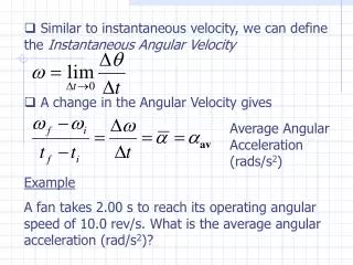
32 x = 2t2 18 x(m) 8 2 0 t(s) 4 3 0 2 1 FYI: Note that the closer the second point is to the first, the closer the slope is to that of the TANGENT line. Topic 2.1 ExtendedA – Instantaneous velocity FYI: In fact, the INSTANTANEOUS VELOCITY at a point on the graph of x vs. t is equal to the SLOPE OF THE TANGENT at that point. As an illustration, suppose we want to know the actual speed the ball at t = 2 s. TANGENT Observe the average velocity as the second point approaches the first (in this case t = 1 s):
x t tA tB FYI: The INSTANTANEOUS VELOCITY is zero where a particle REVERSES direction. FYI: In fact, the INSTANTANEOUS VELOCITY at a point on the graph of x vs. t is equal to the SLOPE OF THE TANGENT at that point. Topic 2.1 ExtendedA – Instantaneous velocity Suppose the x vs. t graph of a particle looks like this: - 0 - - + - 0 (a) Sketch in the instantaneous velocity tangents for various points on the curve: (b) Label the slopes that are zero with a 0: (c) Label the slopes that are negative with a -: (d) Label the slopes that are positive with a +: (e) Label the time where the particle first reverses direction tA: (f) Label the time where the particle next reverses direction tB: