Download
1 / 9
200 likes | 826 Vues
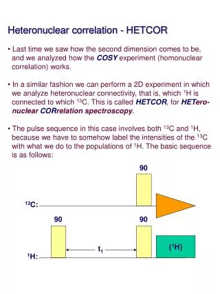
Heteronuclear correlation - HETCOR Last time we saw how the second dimension comes to be, and we analyzed how the COSY experiment (homonuclear correlation) works. In a similar fashion we can perform a 2D experiment in which we analyze heteronuclear connectivity, that is, which 1 H is

E N D
Heteronuclear correlation - HETCOR • Last time we saw how the second dimension comes to be, • and we analyzed how the COSY experiment (homonuclear • correlation) works. • In a similar fashion we can perform a 2D experiment in which • we analyze heteronuclear connectivity, that is, which 1H is • connected to which 13C. This is called HETCOR, for HETero- • nuclear CORrelation spectroscopy. • The pulse sequence in this case involves both 13C and 1H, • because we have to somehow label the intensities of the 13C • with what we do to the populations of 1H. The basic sequence • is as follows: 90 13C: 90 90 {1H} t1 1H:
HETCOR (continued) • We first analyze what happens to the 1H proton (that is, we’ll • see how the 1H populations are affected), and then see how • the 13C signal is affected. For different t1 values we have: z y 90, t1 = 0 90 x x y z y 90, t1 = J / 4 90 x x y z y 90, t1 = 3J / 4 90 x x y
HETCOR (…) • As was the case for COSY, we see that depending on the t1 • time we use, we have a variation of the population inversion • of the proton. We can clearly see that the amount of inversion • depends on the JCH coupling. • Although we did it on-resonance for simplicity, we can easily • show that it will also depend on the 1H frequency (d). • From what we know from SPI and INEPT, we can tell that the • periodic variation on the 1H population inversion will have • the same periodic effect on the polarization transfer to the • 13C. In this case, the two-spin energy diagram is 1H-13C: • Now, since the intensity of the 13C signal that we detect on t2 • is modulated by the frequency of the proton coupled to it, the • 13C FID will have information on the 13C and1H frequencies. 1,2 3,4 bb 13C 4 • • ab 2 1H • • • • • • • • 1H 1,3 2,4 ba ••••• ••••• 3 13C aa I S 1
HETCOR (…) • Again, the intensity of the 13C lines will depend on the 1H • population inversion, thus on w1H. If we use a stacked plot for • different t1 times, we get: • • The intensity of the two • 13C lines will vary with • the w1H and JCH between • +5 and -3 as it did in the • INEPT sequence. • Mathematically, the intensity of one of the 13C lines from the • multiplet will be an equation that depends on w13C on t2 and • w1H on t1, as well as JCH on both time domains: • A13C(t1, t2) trig(w1Ht1) * trig(w13Ct2 ) * trig(JCHt1) * trig(JCHt2) t1 (w1H) w13C f2 (t2)
HETCOR (…) • Again, Fourier transformation on both time domains gives us • the 2D correlation spectrum, in this case as a contour plot: • The main difference in this case is that the 2D spectrum is • not symmetrical, because one axis has 13C frequencies and • the other 1H frequencies. • Pretty cool. Now, we still have the JCH coupling splitting all • the signals of the 2D spectrum in little squares. The JCH are • in the 50 - 250 Hz range, so we can start having overlap of • cross-peaks from different CH spin systems. • We’ll see how we can get rid of them without decoupling (if • we decouple we won’t see 1H to 13C polarization transfer…). w13C JCH w1H f1 f2
HETCOR with no JCH coupling • The idea behind it is pretty much the same stuff we did with • the refocused INEPT experiment. • We use a 13C p pulse to refocus 1H magnetization, and two • delays to to maximize polarization transfer from 1H to 13C • and to get refocusing of 13C vectors before decoupling. As • in INEPT, the effectiveness of the transfer will depend on • the delay D and the carbon type. We use an average value. • We’ll analyze the case of a methine (CH) carbon... 180 90 t1 / 2 t1 / 2 13C: 90 90 {1H} D1 D2 t1 1H:
HETCOR with no JCH coupling (continued) • For a certain t1 value, the 1H magnetization behavior is: • Now, if we set D1 to 1 / 2J both 1H vectors will dephase by • by exactly 180 degrees in this period. This is when we have • maximum population inversion for this particular t1, and no • JCH effects: z y a (w1H - J / 2) 90 t1 / 2 x x a b (w1H + J / 2) b y y y 18013C t1 / 2 x x b b a a z y b 90 D1 x x b a y a
HETCOR with no JCH coupling (…) • Now we look at the 13C magnetization. After the proton p / 2 • we will have the two 13C vectors separated in a 5/3 ratio on • the <z> axis. After the second delay D2 (set to 1 / 2J) they • will refocus and come together: • We can now decouple 1H because the 13C magnetization is • refocused. The 2D spectrum now has no JCH couplings (but • it still has the chemical shift information), and we just see a • single cross-peak where formed by the two chemical shifts: z y y 5 90 D2 x x x 5 5 3 3 y 3 w1H f1 w13C f2
Summary • The HETCOR sequence reports on which carbon is attached • to what proton and shows them both - Great for natural • products stuff. • The way this is done is by inverting 1H population and varying • the transfer of 1H polarization to 13C during the variable t1. • We can obtain a decoupled version by simply lumping in an • refocusing echo in the middle. • Next time • HOMO2DJ spectroscopy. • Coherence transfer and multiple quantum spectroscopy. • HAVE A COOL (AND SAFE) BREAK!!! • (and work on the take-home…)