Download
1 / 1
10 likes | 133 Vues
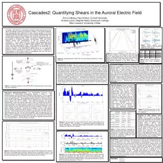
Figure 7: Raw electric and magnetic fields for each payload (FWD blue, AFT green). Figure 4: E/B spectral ratios for two the two orthogonal directions for the AFT payload.

E N D
Figure 7:Raw electric and magnetic fields for each payload (FWD blue, AFT green). Figure 4: E/B spectral ratios for two the two orthogonal directions for the AFT payload. Cascades2: Quantifying Shears in the Auroral Electric FieldErik Lundberg, Paul Kintner, Cornell UniversityKristina Lynch, Meghan Mella, Dartmouth CollegeMarc Lessard, University of New On March, 20th 2009 the Cascades2 sounding rocket was launched from Poker Flat Alaska reaching an apogee of 564km. Two electric/magnetic field subpayloads were ejected at a high velocity parallel to the local magnetic field and included a suite of 3-axis fluxgate magnetometers and crossed dipole electric field antennas with receivers from DC to HF. On the downleg, at altitudes near ~450km, the array of Cascades2 payloads encountered a Poleward Boundary Intensification (PBI) and strong Alfvenic activity with perturbations in the DC electric field of >200mV/m. In this region the two electric field subpayloads were separated by ~6km with a 5 degree angle between their separation vector and the local magnetic field. Initial analysis of the despun DC electric field data differences between payloads of 20 mV/m that are primarily oriented in the East-West direction which at our separation distance of 6km correspond to shears of .0033 mV/m^2. Coupling of these shears to other wave modes is investigated and their role as a possible driver of ion heating is discussed. Figure 6: Cross correlation of the FWD and AFT North DC E signals. Lag indicates by how much time the AFT signal needs to be offset to match the FWD signal (a correlation peak at a positive lag indicates a signal that arrives at the FWD payload first). The inter-payload separation in the North direction is 410m. Figure 3: Unfiltered Electric Fields from The AFT payload overlaid on 0-1KeV electrons. Table 2: Phase velocity estimates derived from cross correlation analysis Correlation Analysis: Figure 6 presents cross correlation analysis, at 3 times spaced before, in, and after the regions of highest shears. The DC electric field is bandpass filtered between .1Hz and 1.5Hz to isolate the lowest frequency waves from DC Electric field. A similar analysis of the east signal has broader peaks at a nearly constant lag of ~.005s (not shown). The plasma velocity is estimated by applying a .1Hz low-pass filter to the DC electric field data and calculating E x B. While realizing this .1Hz cutoff is an arbitrary separation between wave fields and bulk flows, we can calculate the velocity implied by the correlation peaks and the separation between the payloads (dsep/tlag). By subtracting from this the plasma velocity, can calculate a phase velocity. These results are tabulated in Table 2. Notably, the phase velocity in each region is similar in magnitude, but oppositely directed, which we can interpret as either opposite crests of a ~1Hz plane wave, or as the reflection of a plane wave from below the rocket. Quantification of shear: Figures 4 presents electric field data from the AFT payload showing vortex structures. The second panel is a series of 3 hodograms showing the sense of rotation of the electric field in three different time sections, first is counter clockwise around B, second clockwise and third counter clockwise again. The next set of panels present hodograms of the differences between the two payloads during these field reversals. We can convert these differences to velocity through E cross B and then convert those velocities to shear by dividing by the separation between the payloads. This quantification of the shear is exasperated by the need to interpret the differences at spatial or temporal, and, if assuming the differences are spatial whether they are parallel or transverse to B. The space-time ambiguity is discussed later in this poster while different possible values for the shear are presented in Table 1. By assuming the differences are cause by the separation perpendicular field we observe shear frequencies that are appreciable compared to the local O+ cyclotron frequency, fshear/fo+~ .3. Spectral Analysis: Figure 7 presents E over B spectral ratios for the period of interest between 2 and 20Hz. These data are limited by our current magnetometer data reduction which requires high pass filtering of the magnetometer data above 2Hz and is limited by noise above 20Hz. The magnitude of these spectra give us an estimate of the parallel phase velocity of the waves of 1-2*106 m/s which we can extrapolate to lower frequencies, further work is necessary to non-dimensionalize this for comparison to theory, however, we are cautious of using the traditional conversion between space and time (k=omega/vr). Figure 1: Schematic diagram of the CASCADES-2 payloads after all instruments have been deployed. Experiment Setup/Instrumentation: The CASCADES-2 Sounding rocket consisted of 5 instrumented sub-payloads pictured in Figure 1. Two electric/magnetic field sub-payloads are ejected at high velocity (~15 m/s) parallel to the local magnetic field line achieving a parallel separation distance of 8km by the end of flight (Figure 2). These payloads consist of 2 pairs of 12m tip-to-tip wire boom double probes directed radially from the payload’s spin axis which detect plasma waves from DC to 2.4MHz. Two small sub-payloads are ejected perpendicular to the local magnetic field which consist of a single top hat electron detectors designed to observe electrons between .01-5keV along with their pitch-angle distributions. The main payload contains a suite of particle detectors; a pitch angle resolving electron detector observing electrons between .01-5keV, a pitch angle resolving ion detector observing ions between .1-1keV, a field aligned electron detector observing electrons between .01-1keV with very high temporal resolution. All 5 payloads have 3-axis science magnetometers and GPS receivers. Data presented are from the two electric/magnetic field sub-payloads and the electron and ion detectors on the main payload. The relative position between the FWD and AFT subpayloads is presented in figure two. During the time of interest the FWD subpayload is ~6500m above AFT and they’re separation perpendicular to the magnetic field is ~400m (both East and West). Coupling to other plasma wave modes: The 3rd panel of figure 5 presents a spectrogram of electrostatic plasma waves between 20 and 1000Hz. During this active period we observed elevated levels of BBELF noise including emission near the local hyrdogen cyclotron frequency. We note that the largest shears (indicated in the second panel of Figure 5) do not directly line up with the most intense plasma wave emissions, but instead seem to lag slightly behind them. This suggests that the shears and enhanced wave emissions are correlated rather than the shears causing the waves. Figure 4: The top panel is a quiver plot of the DC electric field measured for the AFT payload. The next panel is 3 hodograms spaced throughout the largest field reversal. The third panel displays hodograms of the differences between the FWD and AFT payload. Table 1: Shear frequency estimates for different assumptions about derived from differencing the measured electric fields, converting to velocity through ExB and dividing by separation difference (both parallel and perpendicular). Conclusions: These multipoint measurements of the electric field indicate appreciable shears in the electric field which are maximized on the edges of vortical structures. Shear frequencies of up to 10Hz (corresponding to sheared flows of .37 mV/m2) are observed. During the most active period of flight enhanced BBELF plasma waves are observed along with emission near the local hydrogen gyrofrequency. However, these enhanced plasma waves don’t necessarily correlate with the periods of the highest shear. The temporal evolution of these waves are studied via cross correlation analysis, which reveals oscillating wave fields that reach up to 8000km/s for the frequency range between .1-1.5Hz. Parallel phase velocity is estimated to be 1-2*106m/s from |E/deltaB|, which is consistent the temporal delay in the Eastward electric field signals (not shown). Further work is needed to elucidate the connections between structured precipitating electrons and electric fields, the observed waves and fields and accelerated ions. Figure 2: Separation distance between the two electric field subpayloads in Vertical-East-North coordinates where vertical is transformed to be parallel to local B. The first panel covers the entire flight while the second and third panels focus on the along B and perpendicular to B separations during the period of interest. Figure 5: The top two panels are quiver plots of the AFT DC electric field and the differences between the FWD and AFT electric fields respectively. The third plot is a frequency-time spectrogram of the VLF12 channel of the AFT payload indicated enhanced BBELF waves and enhanced emissions near the local hydrogen gyrofrequency (~535 Hz). Contact: Erik Lundberg Etl22@cornell.edu 301 Rhodes Hall Cornell University Ithaca, NY 14853