Download

1 / 31
350 likes | 645 Vues
Occupational Air Sampling Strategies – who, when, how…. Lecture Notes. Components of a Sampling Strategy. Characterization and information gathering Risk assessment and sampling priorities Air sampling strategy and analysis Data interpretation Recommendation and reporting Re-evaluation.

E N D
Occupational Air Sampling Strategies – who, when, how…. Lecture Notes
Components of a Sampling Strategy • Characterization and information gathering • Risk assessment and sampling priorities • Air sampling strategy and analysis • Data interpretation • Recommendation and reporting • Re-evaluation
Air sampling strategy • Which employee or employees should be sampled? • How many samples should be taken on each workday sampled to define the employee’s exposure? • How long should the sampling interval be for a measurement sample?
Air sampling strategy • What periods during the workday should the employee’s exposure be sampled? • How many workdays during the year should be sampled and when? • Time to result – acute vs. chronic and direct reading real time vs. sampling media and two-week lab time.
Which employee or employees should be sampled? • OSHA regulation requires the sampling of the “employee believed to have the greatest exposure” or the “maximum risk employee” - principle extended to include groups of employees • Use the exposure risk/health risk priority matrix
Which employee or employees should be sampled? • If the maximum risk employee or group can’t be identified then do random sampling of the group of workers. • Objective is to select a subgroup of adequate size so that there is a high probability that the random sample will contain at least one worker with high exposure if one exists. • Want to be careful about use of group statistics
NIOSH’s Occupational Exposure Sampling Strategies Manual • Gives one sample size model • Set up to ensure with 90% confidence that at least one person from the highest 10% exposure group is contained in the sample • Conversely 10% chance of missing someone in the highest 10% exposure group
Samplingperiods • Various types of sampling periods possible • As you increase the # of sample periods in a shift the analysis becomes more sophisticated
How many workdays during the year should be sampled and when? • OSHA regulation can differ • Substance specific standards specify sample interval dependent on the exposure level relative to the PEL
1910.1025 Lead • 1910.1025(c)(1) The employer shall assure that no employee is exposed to lead at concentrations greater than fifty micrograms per cubic meter of air (50 mg/m3) averaged over an 8-hour period. • 1910.1025(c)(2) If an employee is exposed to lead for more than 8 hours in any work day, the permissible exposure limit, as a time weighted average (TWA) for that day, shall be reduced according to the following formula: • Maximum permissible limit (in mg/m3)=400 divided by hours worked in the day.
1910.1025 Lead • 1910.1025 (d) Exposure monitoring - • 1910.1025(d)(1)(ii) With the exception of monitoring under paragraph (d)(3), the employer shall collect full shift (for at least 7 continuous hours) personal samples including at least one sample for each shift for each job classification in each work area. • 1910.1025(d)(1)(iii) Full shift personal samples shall be representative of the monitored employee's regular, daily exposure to lead.
1910.1025 Lead • 1910.1025(d)(2) Initial determination. Each employer who has a workplace or work operation covered by this standard shall determine if any employee may be exposed to lead at or above the action level. • 1910.1025(d)(4)(i) Where a determination conducted under paragraphs (d)(2) and (3) of this section shows the possibility of any employee exposure at or above the action level, the employer shall conduct monitoring which is representative of the exposure for each employee in the workplace who is exposed to lead.
1910.1025 Lead • 1910.1025(d)(6) Frequency. • 1910.1025(d)(6)(i) If the initial monitoring reveals employee exposure to be below the action level the measurements need not be repeated except as otherwise provided in paragraph (d)(7) of this section. • 1910.1025(d)(6)(ii) If the initial determination or subsequent monitoring reveals employee exposure to be at or above the action level but below the permissible exposure limit the employer shall repeat monitoring in accordance with this paragraph at least every 6 months. The employer shall continue monitoring at the required frequency until at least two consecutive measurements, taken at least 7 days apart, are below the action level at which time the employer may discontinue monitoring for that employee except as otherwise provided in paragraph (d)(7) of this section.
1910.1025 Lead • 1910.1025(d)(6)(iii) If the initial monitoring reveals that employee exposure is above the permissible exposure limit the employer shall repeat monitoring quarterly. The employer shall continue monitoring at the required frequency until at least two consecutive measurements, taken at least 7 days apart, are below the PEL but at or above the action level at which time the employer shall repeat monitoring for that employee at the frequency specified in paragraph (d)(6)(ii), except as otherwise provided in paragraph (d)(7) of this section. • 1910.1025(d)(7) Additional monitoring. Whenever there has been a production, process, control or personnel change which may result in new or additional exposure to lead, or whenever the employer has any other reason to suspect a change which may result in new or additional exposures to lead, additional monitoring in accordance with this paragraph shall be conducted.
Limited basic statistics review • What is a population? • All of something, e.g. • A lot of silicon wafers produced in a semiconductor factory • The 2003 semester students in IH&S 725 • All lead exposures to “metal pourers” • What is a sample? • Observations selected from a larger population • A sample of the silicon wafers from a lot • A sample of students from the 2003 IH&S 725 class • A sample of lead exposures from all possible exposures
Variance and standard deviation Population Sample
Point estimate • A point estimate of some population parameter is a single numerical value of a statistic • Sample mean is a point estimate of an unknown population mean • Sample variance is a point estimate of an unknown population variance
2-sided confidence interval on the mean • Two sided CI • P(L ≤ µ ≤ U) = 1-α where 0 ≤ α ≤ 1 • We have a probability of 1-α of selecting a sample that will produce a interval containing the true value of µ • The interval l≤ µ ≤ u is called a 100(1-α) percent confidence interval • I and u are the lower- and upper-confidence limits • (1-α) is the confidence coefficient
Confidence Interval on sample mean: One-sided Confidence Interval • α is assigned to either the upper or lower tail of the t-distribution
Where does t come from • Definition • Let X1X2 ….Xn be a random sample for a normal distribution with unknown mean and unknown variance σ2. The quantity has a t-distribution with n-1 degrees of freedom.
t-distribution and α • Probability density function i.e.. area under the curve = 1. • α represents the area assigned to the tail(s) of the distribution – probability of T > t1-α &/or -tα • Note that t1-α = -tα
Example #1 • Using the t-table determine the t-value with 14 df that leaves an area of 0.025 to the left (and therefore an area of 0.975 to the right).
Example #2 • What is the P(-t0.025 < T < t0.025)? • Since t0.025 leaves an area of 0.025 to the right and -t0.025 leaves and area of 0.025 to the left the total area (probability) between -t0.025 and t0.025 is? 1- 0.025 – 0.025 = 0.95
Influence of degrees of freedom on the t-distribution • The area to the left or right of tα and t1-α decreases with increasing df • Note from the t-table that as df gets large it the t-value approaches the z value from the SND table
Standard normal distribution, SND • Definition • If is the mean of a random sample of size n taken from a population with mean µ and variance σ2, then the limiting form of the distribution of: as n ∞, is the standard normal distribution snd(z;0,1).
Using the standard normal distribution • Using the z-table, find the area under the curve that lies: • to the right of z = 1.84 • 1- area to the left of z = 1.84 • 1-0.9671= 0.0329 or 3.29% • between z = -1.97 and z = 0.86 • 0.8051 - 0.0244 = 0.7807
Example #3 • Given a normal distribution with µ = .05mg/m3 and σ = 0.01, find the probability that a sample point estimate of µ would fall between 0.04 and 0.06mg/m3.
Example #3 solution • First calculate the z-value corresponding to x1 = .04mg/m3 and x2 = .06mg/m3
Example #3 solution con’t • Second determine the probability • P(0.04mg/m3 < x < 0.06mg/m3) = P(-1< z < 1)