Understanding Consumer Behavior in Revenue Management: A Choice-Based Model Approach
This paper explores the significance of consumer behavior modeling in revenue management (RM) and inventory control. It highlights the limitations of traditional models that assume independent demand, emphasizing the impact of consumer choice on pricing and inventory decisions. The authors present a choice-based model, discussing its formulation through dynamic programming and its applicability to airline ticket pricing strategies. By examining variables such as demand volatility, customer segments, and fare choices, the study aims to improve revenue strategies through a refined understanding of consumer behavior.

Understanding Consumer Behavior in Revenue Management: A Choice-Based Model Approach
E N D
Presentation Transcript
Consumer Behavior Modeling Linling He, Xiaoyan Liu, and Muhong Zhang April 29, 2005
Consumer Behavior Modeling Outlines • Choice-Based Model in Revenue Management • Literature Review in Inventory Competition Model • Choice based inventory competition Model
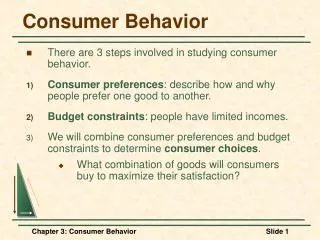
Why Model Consumer Behavior? • Usually in RM or inventory control, we start our analysis with some set of assumptions assuming an underlying stochastic or deterministic demand process • What if… • assumptions are incorrect • our model parameters are unknown?
Why Model Consumer Behavior? (cont) • Example: • Two classes of tickets (low/high fares) • Flexible customer, but buys low fare when available • An air-line chooses reserve level for the high-fare tickets based on historical data on sales • What happens if we neglect to account for consumer’s choice behavior? “Spiral Down Effect”
Choice-Based Model in Revenue Management • History • Motivation for choice modeling • Single-leg Model • Dynamic Programming Formulation • Network RM Model • Dynamic Programming Formulation • Deterministic LP Formulation • Asymptotic optimality
1.1 What is Revenue Management? • Before 1972: controlled booking • Around 70’s: discount/full fare seat inventory control • Littlewood (1972) marked the beginning of Yield Management. “…Discount fare booking should be accepted as long as their revenue value exceeded the expected revenue of future full fair bookings…” • Single-leg control, segment control, origin-destination control
1.1 What is Revenue Management? (cont) • Practice of controlling the availability and/or pricing of travel seats in different booking classes with the goal of maximizingexpected revenues or profits. • Fundamental revenue management decision: whether or not to accept or reject this booking • Key areas of research • Forecasting • Overbooking • Seat inventory control • pricing
Consumer Behavior and Demand Forecasting Demand volatility Sensitivity to pricing actions Demand dependencies btwn different booking classes Control System Booking lead time Overbooking Leg-based, segment-based, or full ODF control Revenue Factors Fare values Frequent flyer redemptions Cancellation penalties or restrictions Variable Cost Factors Marginal costs per passenger Denied boarding penalties Problem Scale Large airline or airline alliance 1.1 What is Revenue Management (cont)
1.2 Motivation for Choice Modeling (cont) • Choices among fare products Flight AB123 Y $320 Unrestricted Q $189 Nonrefundable
1.2 Motivation for Choice Modeling (cont) • Choice among multiple departure times between same OD 6:50 AM Open: Y, M, B, Q 9:15 AM Open: Y, M Closed: Q, B 1:10 PM Open: Y, M, B Closed: Q
1.2 Motivation for Choice Modeling (cont) • Choice among different routing Long Beach Q class, connecting flight $179 New York Q Class: nonstop flight $154 Oakland
1.2 Motivation for Choice Modeling • Traditional model: • Demand is mutually statistically independent and also unaffected by the availability control. • Heuristic correction: “buy-up”“buy-down” • But, traditional RM techniques are limited! • More over… • Competition is fundamentally about choice… • It is natural to consider Consumer Behavior Models!
1.3 Single-leg Model • Traditional Model (At most one arrival per period)
1.3 Single-leg Model (cont) • Discrete DP Formulation
Bid price decision rule: Open class j iff… 1.3 Single-leg Model (cont) Open class j if the revenue of class j is greater than or equal to the marginal value of extra capacity
aircraft cabin 1.3 Single-leg Model (cont) • Nested allocation decision rule: i nested protection level for class i or higher
1.3 Single-leg Model (cont) • Traditional model assumes a arrival pattern for class j, does not consider consumer’s choice • In reality, each customer makes a choice among the fare products that are offered (Talluj and van Ryzin) • Control decision now: which products do we make available?
1.3 Single-leg Model (cont) • Example • Discounts: • Customer Segments:
1.3 Single-leg Model (cont) • Each offer set leads to a different outcome… Ex. If we offer the full fare (Y) and the 21-Day advance purchase discount (M), then 10% buy full fare (Y) 40% buy 21-Day discount (M) 50% do not buy Why?
1.3 Single-leg Model (cont) • The revised single-leg model
1.3 Single-leg Model (cont) • Revised choice-based DP t time remaining x number of seats remaining Vt(x) value function Pj(S)probability of choosing j given offer set S Bellman’s Equation: (1)
1.3 Single-leg Model (cont) • Efficient Sets: A set T is said to be inefficient if a mixture of other offer sets can be used to generate more revenue for the same (or lower consumption rate. Mathematically: set of convex weights (S), SN satisfying S (S)=1 and (S)>=0, SN such that R(T)< S (S)R(S) Q(T) S (S)Q(S) R(S)=expected revenue Q(S)=probability of selling a unit using offer set S
1.3 Single-leg Model (cont) An optimal policy: • select a set k*from among the m efficient, ordered sets {Sk: k=1,…m}, where S1S2… Sm that maximizes (1). • For a fixed t, the largest optimal index k* is increasing in the remaining capacity x, • For any fixed x, k* is decreasing in the remaining time t.
An “efficient frontier inefficient offer sets 3 efficient combinations: {Y}, {Y,Q}, {Y,Q,M} These are the only combinations we should consider!
More capacity/ Less time Less capacity/ more time 1.3 Single-Leg Model (cont) • Optimal policy: Use efficient sets in this order as capacity / time change Optimal policy: Use efficient sets in this order as capacity/time change
1.3 Single-leg Model (cont) • Notice what’s “odd” in this example! • It can be optimal to offer deep discount (Q) but NOT the moderate discount (M). Why? • Some business customers who buy the full fare may “buy-down” to M if it is offered • Leisure customers will not buy full fare anyway • Numerical examples show revenue benefits over standard methods can be very large.
1.3 Single-leg Model (cont) • A variety of choice models can be used… • MNL (The ratio of the probabilities of any two alternatives is independent from the choice set.) • But there are many other possibilities… • Finite mixture logit • Nested logit • General random utility
1.4 Network RM Model (cont) m = no. of legs n = no. of products (itinerary x fare-class combo) N = {1,…n}=set of all products c = (c1,…cm)=initial capacity rj = revenue of fare-product j A = [aij]mxn=incidence matrix (aij=1 if leg i is use for product j) Aj = incidence vector for product j Ai = incidence vector for leg I = prob. Of an arrival in each time period
1.4 Network RM Model (cont) Control: set of products to make available at each point in time, i.e. offer set, SN Pj(S) = prob. of arriving customer chooses fare-product j given offer set S P0(S) = prob. Of no purchase jSPj(S)+P0(S)=1 Decision: find an optimal policy for choosing the offer set S at each time t and giving the remaining capacity x such that their total expected revenue is maximized.
1.4 Network RM Model (cont) • Dynamic Programming formulation Boundary Conditions: Vt(0)=0 t=1,…,T VT+1(x)=0 x0
1.4 Network RM Model (cont) • DP not solvable for most realistic network due to the large dimensionality of the state space • Use Deterministic Approximation with stochastic quantities replaced by mean values and assume continuous capacities and demand
1.4 Network RM Model (cont) • R(S) = expected revenue from an arriving customer when S is offered. • P(S)=vector of purchase probabilities • Qi(S) = probability of using a unit of capacity on leg i, i=1,…,m, given S.
1.4 Network RM Model (cont) • Choice-Based Deterministic LP (CDLP) Max. total revenue Consumption less than capacity Total time sets offered less than horizon length S = subset of available (open) products (the offer set) Decision variables:t(S) = Total time subset S is offered
1.4 Network RM Model (cont) • This LP has an exponential number of variables! How do we solve it? • Gallego et al. show for special classes of choice models, LP can be solved relatively efficiently using column generation Ex: Customers belong to L segment and each segment l • Has a disjoint consideration setCl • Makes multinomial logit (MNL) choice among products in Cl Then columns can be generated by a simple ranking procedure (linear complexity in |Cl|)
1.4 Network RM Model (cont) Asymptotic optimality (van Ryzin & Liu 2004) Theorem: Consider scaled problem in which capacity and time are both increased by the same factor q…. Let t*(S)denote the optimal solution to the original choice-based LP. Then the solution qt*(S) is asymptotically optimal for the corresponding stochastic dynamic network choice problem (suitably defined). Capacity= qx Time horizon=qT
1.4 Network RM Model (cont) • How do we use the choice-based DLP solution? • Directly apply time variables t*(S) (Gallego et al. 2004) • Discard primal solution, but use dual information in a decomposition heuristic and other analysis (van Ryzin & Liu 2004)
1.4 Network RM Model (cont) • Dual of CDLP:
1.4 Network RM Model (cont) • Prop. 3 A set T is efficient if and only if for some =(1,…,m)t0, T is the optimal solution to maxS{R(S)- tQ(S)}. • Prop. 4 If t*(T)>0 in the optimal solution to the CDLP, then T is an efficient set. • Prop. 5 If Q(S2)Q(S1), then R(S2) R(S1). • Efficient sets are partially order. (compare to the single-leg problem)
1.4 Network RM Model (cont) • Can solution to Single-leg RM problem be applied to Network RM? • Vt-1(x)-Vt-1(x-Aj) is not additive in Aj • In general, efficient sets are not the only optimal solution to the original DP. • Special case: additivity property holds if each product uses only a single leg • But, by our Asymptotic optimality condition, the efficient sets are asymptotically optimal for the DP.
1.4 Network RM Model (cont) Simulation-based optimization in network RM Basic Idea: • Define a parametric class of policies (e.g. booking limit, bid price) • Use simulation and sensitivity information to optimize the policy parameters.
Consumer Behavior Modeling Outlines • Choice-Based Model in Revenue Management • Literature Review in Inventory Competition Model • Choice based inventory competition Model
Outline – Literature Review on Inventory Competition • Parlar (1988) – 2-firm model • Existence and Uniqueness of NE • Maxmin strategy • Cooperation between players • Lippman and McCardle (1994) • Results on 2-firm model • Summary of N-firm model
2.1 Literature Review in Inventory Competition Model Parlar (1988) - 2-Firm Model Existence of NE Uniqueness of NE Maxmin strategy Cooperation between players
Literature Review in Inventory Competition Model 2-Firm Model Assumptions: • Single period, Single product • Independent random demand at each firm • Substitution of products allowed • Deterministic fraction of excess demand substitutes to alternatives • No price competition • Continuous and strictly increasing CDF
Literature Review in Inventory Competition Model Notations: • pi : shortage cost/unit for firm i’s product • si: sales price/unit of firm i’s product • ci: order cost/unit for firm i’s product • qi: savage value of firm i’s product • Di: random demand of firm i’s product ~ Fi(y) • bi: fraction of firm i’s demand which will switch to firm j’s product when it is sold out at firm i • xi: order quantity of each firm
Literature Review in Inventory Competition Model Player i’s Expected Profit Function: Sales price Savage value Penalty cost Order cost
Comparison • Recall the game theory version of the newsvendor model introduced in class in week 8. • It is a compact version of Parlar’s model without two terms: savage value and penalty cost. Also, bi is set to be one. • Conclusion on that model: the expected profit function is concave, and by Theorem (Debrea, 1952), there exists at least one pure strategy NE in the game.