Download
1 / 19
190 likes | 612 Vues
Learning Objectives for Section 14.1 Area Between Two Curves. The student will be able to Determine the area between a curve and the x axis , Determine the area between two curves, and 3. Solve an application involving income distribution. . Negative Values for the Definite Integral.

E N D
Learning Objectives for Section 14.1 Area Between Two Curves • The student will be able to • Determine the area between a curve and the x axis , • Determine the area between two curves, and • 3. Solve an application involving income distribution. Barnett/Ziegler/Byleen Business Calculus 11e
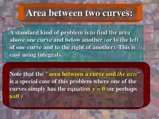
Negative Values for the Definite Integral If f (x) is positive for some values of x on [a, b] and negative for others, then the definite integral y = f (x) is the cumulative sum of the signed areas between the graph of f (x) and the x axis. Areas above the x axis are positive, and areas below are negative. In this section we want find the (unsigned) actual area between a curve and the x axis or between two curves. This is never negative! B a A b Barnett/Ziegler/Byleen Business Calculus 11e
Negative Values The (unsigned) area between the graph of a negative function and the x axis is equal to the definite integral of the negative of the function. y = f (x) B a A b c Barnett/Ziegler/Byleen Business Calculus 11e
Area Between Curve and x axis The area between f (x) and the x axis can be found as follows: For f (x) 0 over [a, b] (i.e. f (x) is above the x axis): Area = For f (x) 0 over [a, b] (i.e. f (x) is below the x axis): Area = Barnett/Ziegler/Byleen Business Calculus 11e
A 1 A 2 Example Find the area bounded by y = 4 – x2; y = 0, 1 x 4. Barnett/Ziegler/Byleen Business Calculus 11e
A 1 A 2 Example Find the area bounded by y = 4 – x2; y = 0, 1 x 4. Area = A1 - A2 Barnett/Ziegler/Byleen Business Calculus 11e
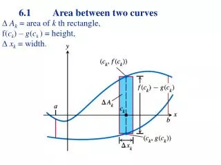
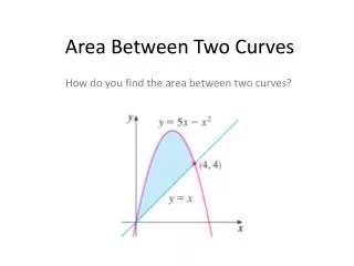
Area Between Two Curves Theorem 1. If f (x) g(x) over the interval [a, b], then the area bounded by y = f (x) and y = g(x) for a x b is given by f (x) A g (x) a b Barnett/Ziegler/Byleen Business Calculus 11e
Example Find the area bounded by y = x2 – 1 andy = 3. Barnett/Ziegler/Byleen Business Calculus 11e
Example Find the area bounded by y = x2 – 1 andy = 3. Note the two curves intersect at –2 and 2, and y = 3 is the larger function on –2 x 2. Barnett/Ziegler/Byleen Business Calculus 11e
Computing Areas Using a Numerical Integration Routine Suppose we want to find the area bounded by Barnett/Ziegler/Byleen Business Calculus 11e
Computing Areas Using a Numerical Integration Routine Suppose we want to find the area bounded by First, we use a graphing calculator to graph the functions f and g and find their intersection points as in the figure. We see that the graph of f is bell shaped and the graph of g is a parabola, and that f (x) >g(x) on the interval [-1.131, 1.131]. Barnett/Ziegler/Byleen Business Calculus 11e
Computing Areas Using a Numerical Integration Routine Then we compute the area by a numerical integration routine on a calculator. Barnett/Ziegler/Byleen Business Calculus 11e
Application: Income Distribution The U.S. Bureau of the Census compiles data on distribution of income among families. This data can be fitted to a curve using regression analysis. This curve is called a Lorenz curve. The variable x represents the cumulative percentage of families at or below the given income level. The variable y represents the cumulative percentage of total family income received. If we have absolute equality of income (every family has the same income), the Lorenz curve is y = x. Barnett/Ziegler/Byleen Business Calculus 11e
Application(continued) Curve of absolute equality y = x For example, data point (approximately) (0.4, 0.09) in the table indicates that the bottom 40% of families receive only 9% of the total income for all families. Data point (.6, .26) indicates that the bottom 60% of families receive only 26% of the total income, etc. Lorenz Curve (0.4, 0.09) Barnett/Ziegler/Byleen Business Calculus 11e
Application(continued) If we have absolute inequality of income (one family has all the income, the rest have none), the Lorenz curve is y(x) = 0 for x < 1, y(1) = 1. The maximum possible area between the Lorenz curve and the line y = x is ½, which occurs in the case of absolute inequality. That is, the area between the Lorenz curve and the line y = x is between 0 and ½. The Gini Index is two times the area between the Lorenz curve and the line y = x. It can take on values between 0 and 1. Barnett/Ziegler/Byleen Business Calculus 11e
Application(continued) Gini Index of Income Concentration If y = f (x) is the Lorenz curve, then Index of income concentration = A measure of 0 indicates absolute equality. A measure of 1 indicates absolute inequality. Barnett/Ziegler/Byleen Business Calculus 11e
Example A country is planning changes in tax structure in order to provide a more equitable distribution of income. The two Lorenz curves are: f (x) = x2.3 currently, and g(x) = 0.4x + 0.6x2 proposed. Will the proposed changes work? Barnett/Ziegler/Byleen Business Calculus 11e
Example(continue) Currently: Gini Index of income concentration = Future: Gini Index of income concentration = The Gini index is decreasing, so the future distribution will be more equitable. Barnett/Ziegler/Byleen Business Calculus 11e
Summary • We reviewed the definite integral as the area between a curve and the x axis. • We learned how to calculate area when the curve was below the x axis. • We learned how to calculate the area between two curves. • We learned about the Lorenz curve and the Gini index of income concentration. Barnett/Ziegler/Byleen Business Calculus 11e