Independence : Events A and B are independent if

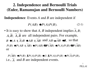
1. 2. Independence and Bernoulli Trials (Euler, Ramanujan and Bernoulli Numbers) • Independence: Events A and B are independent if • It is easy to show that A, B independent implies • are all independent pairs. For example, • and so that • or • i.e., and B are independent events. (2-1) PILLAI

2. As an application, let Ap and Aq represent the events and Then from (1-4) Also Hence it follows that Ap and Aq are independent events! (2-2) PILLAI

3. If P(A) = 0, then since the event always, we have • and (2-1) is always satisfied. Thus the event of zero • probability is independent of every other event! • Independent events obviously cannot be mutually • exclusive, since and A, B independent • implies Thus if A and B are independent, • the event AB cannot be the null set. • More generally, a family of events are said to be • independent, if for every finite sub collection • we have (2-3) PILLAI

4. Let • a union of n independent events. Then by De-Morgan’s • law • and using their independence • Thus for any A as in (2-4) • a useful result. • We can use these results to solve an interesting number theory problem. (2-4) (2-5) (2-6) PILLAI

5. Example 2.1: Three switches connected in parallel operate independently. Each switch remains closed with probability p. (a) Find the probability of receiving an input signal at the output. (b) Find the probability that switch S1 is open given that an input signal is received at the output. Solution: a. Let Ai = “Switch Si is closed”. Then Since switches operate independently, we have Input Output Fig.2.1 PILLAI

6. Let R = “input signal is received at the output”. For the event R to occur either switch 1 or switch 2 or switch 3 must remain closed, i.e., (2-7) Using (2-3) - (2-6), (2-8) We can also derive (2-8) in a different manner. Since any event and its compliment form a trivial partition, we can always write (2-9) But and and using these in (2-9) we obtain (2-10) which agrees with (2-8). PILLAI

7. Note that the events A1, A2, A3 do not form a partition, since they are not mutually exclusive. Obviously any two or all three switches can be closed (or open) simultaneously. Moreover, b. We need From Bayes’ theorem Because of the symmetry of the switches, we also have (2-11) PILLAI

8. Repeated Trials Consider two independent experiments with associated probability models (1, F1, P1) and (2, F2, P2). Let 1, 2 represent elementary events. A joint performance of the two experiments produces an elementary events  = (, ). How to characterize an appropriate probability to this “combined event” ? Towards this, consider the Cartesian product space  = 1 2 generated from 1 and 2 such that if   1 and   2 , then every  in  is an ordered pair of the form  = (, ). To arrive at a probability model we need to define the combined trio (, F, P). PILLAI

9. Suppose AF1 and B  F2. Then A  B is the set of all pairs (, ), where   A and   B. Any such subset of  appears to be a legitimate event for the combined experiment. Let F denote the field composed of all such subsets A  B together with their unions and compliments. In this combined experiment, the probabilities of the events A  2 and 1  B are such that Moreover, the events A  2 and 1  B are independent for any A  F1 and B  F2 . Since we conclude using (2-12) that (2-12) (2-13) PILLAI

10. (2-14) for all A  F1 and B  F2. The assignment in (2-14) extends to a unique probability measure on the sets in F and defines the combined trio (, F, P). Generalization: Given n experiments and their associated let represent their Cartesian product whose elementary events are the ordered n-tuples where Events in this combined space are of the form where and their unions an intersections. (2-15) (2-16) PILLAI

11. If all these n experiments are independent, and is the probability of the event in then as before Example 2.3: An event A has probability p of occurring in a single trial. Find the probability that A occurs exactly k times, k  n in n trials. Solution: Let (, F, P) be the probability model for a single trial. The outcome of n experiments is an n-tuple where every and as in (2-15). The event A occurs at trial # i , if Suppose A occurs exactly k times in . (2-17) (2-18) PILLAI

12. Then k of the belong to A, say and the remaining are contained in its compliment in Using (2-17), the probability of occurrence of such an  is given by However the k occurrences of A can occur in any particular location inside . Let represent all such events in which A occurs exactly k times. Then But, all these s are mutually exclusive, and equiprobable. (2-19) (2-20) PILLAI

13. Thus where we have used (2-19). Recall that, starting with n possible choices, the first object can be chosen n different ways, and for every such choice the second one in ways, … and the kth one ways, and this gives the total choices for k objects out of n to be But, this includes the choices among the k objects that are indistinguishable for identical objects. As a result (2-21) (2-22) PILLAI

14. represents the number of combinations, or choices of n identical objects taken k at a time. Using (2-22) in (2-21), we get a formula, due to Bernoulli. Independent repeated experiments of this nature, where the outcome is either a “success” or a “failure” are characterized as Bernoulli trials, and the probability of k successes in n trials is given by (2-23), where p represents the probability of “success” in any one trial. (2-23) PILLAI

15. Example 2.4: Toss a coin n times. Obtain the probability of getting k heads in n trials ? Solution: We may identify “head” with “success” (A) and let In that case (2-23) gives the desired probability. Example 2.5: Consider rolling a fair die eight times. Find the probability that either 3 or 4 shows up five times ? Solution: In this case we can identify Thus and the desired probability is given by (2-23) with and Notice that this is similar to a “biased coin” problem. PILLAI

16. Bernoulli trial: consists of repeated independent and identical experiments each of which has only two outcomes A or with and The probability of exactly k occurrences of A in n such trials is given by (2-23). Let Since the number of occurrences of A in n trials must be an integer either must occur in such an experiment. Thus But are mutually exclusive. Thus (2-24) (2-25) PILLAI

17. Fig. 2.2 (2-26) From the relation (2-26) equals and it agrees with (2-25). For a given n and p what is the most likely value of k ? From Fig.2.2, the most probable value of k is that number which maximizes in (2-23). To obtain this value, consider the ratio (2-27) PILLAI

18. (2-28) Thus if or Thus as a function of k increases until if it is an integer, or the largest integer less than and (2-29) represents the most likely number of successes (or heads) in n trials. Example 2.6: In a Bernoulli experiment with n trials, find the probability that the number of occurrences of A is between and (2-29) PILLAI

19. Solution: With as defined in (2-24), clearly they are mutually exclusive events. Thus Example 2.7: Suppose 5,000 components are ordered. The probability that a part is defective equals 0.1. What is the probability that the total number of defective parts does not exceed 400 ? Solution: Let (2-30) PILLAI

20. Using (2-30), the desired probability is given by Equation (2-31) has too many terms to compute. Clearly, we need a technique to compute the above term in a more efficient manner. From (2-29), the most likely number of successes in n trials, satisfy or (2-31) (2-32) (2-33) PILLAI

21. so that From (2-34), as the ratio of the most probable number of successes (A) to the total number of trials in a Bernoulli experiment tends to p, the probability of occurrence of A in a single trial. Notice that (2-34) connects the results of an actual experiment ( ) to the axiomatic definition of p. In this context, it is possible to obtain a more general result as follows: Bernoulli’s theorem: Let A denote an event whose probability of occurrence in a single trial is p. If k denotes the number of occurrences of A in n independent trials, then (2-34) (2-35) PILLAI

22. Equation (2-35) states that the frequency definition of probability of an event and its axiomatic definition ( p) can be made compatible to any degree of accuracy. Proof: To prove Bernoulli’s theorem, we need two identities. Note that with as in (2-23), direct computation gives Proceeding in a similar manner, it can be shown that (2-36) (2-37) PILLAI

23. Returning to (2-35), note that which in turn is equivalent to Using (2-36)-(2-37), the left side of (2-39) can be expanded to give Alternatively, the left side of (2-39) can be expressed as (2-38) (2-39) (2-40) (2-41) PILLAI

24. Using (2-40) in (2-41), we get the desired result Note that for a given can be made arbitrarily small by letting n become large. Thus for very large n, we can make the fractional occurrence (relative frequency) of the event A as close to the actual probability p of the event A in a single trial. Thus the theorem states that the probability of event A from the axiomatic framework can be computed from the relative frequency definition quite accurately, provided the number of experiments are large enough. Since is the most likely value of k in n trials, from the above discussion, as the plots of tends to concentrate more and more around in (2-32). (2-42) PILLAI

25. Next we present an example that illustrates the usefulness of “simple textbook examples” to practical problems of interest: Example 2.8 : Day-trading strategy : A box contains n randomly numbered balls (not 1 through n but arbitrary numbers including numbers greater than n). Suppose a fraction of those balls are initially drawn one by one with replacement while noting the numbers on those balls. The drawing is allowed to continue until a ball is drawn with a number larger than the first m numbers. Determine the fraction p to be initially drawn, so as to maximize the probability of drawing the largest among the n numbers using this strategy. Solution: Let “ drawn ball has the largest number among all n balls, and the largest among the PILLAI

26. first k balls is in the group of first m balls, k > m.” (2.43) Note that is of the form where A = “largest among the first k balls is in the group of first m balls drawn” and B = “(k+1)st ball has the largest number among all n balls”. Notice that A and B are independent events, and hence Where m = np represents the fraction of balls to be initially drawn. This gives P (“selected ball has the largest number among all balls”) (2-44) (2-45)

27. Maximization of the desired probability in (2-45) with respect to p gives or From (2-45), the maximum value for the desired probability of drawing the largest number equals 0.3679 also. Interestingly the above strategy can be used to “play the stock market”. Suppose one gets into the market and decides to stay up to 100 days. The stock values fluctuate day by day, and the important question is when to get out? According to the above strategy, one should get out (2-46) PILLAI

28. at the first opportunity after 37 days, when the stock value exceeds the maximum among the first 37 days. In that case the probability of hitting the top value over 100 days for the stock is also about 37%. Of course, the above argument assumes that the stock values over the period of interest are randomly fluctuating without exhibiting any other trend. Interestingly, such is the case if we consider shorter time frames such as inter-day trading. In summary if one must day-trade, then a possible strategy might be to get in at 9.30 AM, and get out any time after 12 noon (9.30 AM + 0.3679 6.5 hrs = 11.54 AM to be precise) at the first peak that exceeds the peak value between 9.30 AM and 12 noon. In that case chances are about 37% that one hits the absolute top value for that day! (disclaimer : Trade at your own risk) PILLAI

29. Game of Craps • A pair of dice is rolled on every play, • Win: sum of the first throw is 7 or 11 • Lose: sum of the first throw is 2, 3, 12 • Any other throw is a “carry-over” • If the first throw is a carry-over, then the player throws the dice repeatedly until: • Win: throw the same carry-over again • Lose: throw 7 Find the probability of winning the game.

30. Game of Craps P1: the probability of a win on the first throw Q1: the probability of loss on the first throw B: winning the game by throwing the carry-over C: throwing the carry-over

31. Game of Crap The probability of win by throwing the number of Plays that do not count is: The probability that the player throws the carry-over k on the j-th throw is:

32. Game of Crap

33. Example 2.9: Game of craps using biased dice: From Example 3.16, Text, the probability of winning the game of craps is 0.492929 for the player. Thus the game is slightly advantageous to the house. This conclusion of course assumes that the two dice in question are perfect cubes. Suppose that is not the case. Let us assume that the two dice are slightly loaded in such a manner so that the faces 1, 2 and 3 appear with probability and faces 4, 5 and 6 appear with probability for each dice. If T represents the combined total for the two dice (following Text notation), we get PILLAI

34. (Note that “(1,3)” above represents the event “the first dice shows face 1, and the second dice shows face 3” etc.) For we get the following Table: PILLAI

35. This gives the probability of win on the first throw to be (use (3-56), Text) and the probability of win by throwing a carry-over to be (use (3-58)-(3-59), Text) Thus Although perfect dice gives rise to an unfavorable game, (2-47) (2-48) (2-49) PILLAI

36. a slight loading of the dice turns the fortunes around in favor of the player! (Not an exciting conclusion as far as the casinos are concerned). Even if we let the two dice to have different loading factors and (for the situation described above), similar conclusions do follow. For example, gives (show this) Once again the game is in favor of the player! Although the advantage is very modest in each play, from Bernoulli’s theorem the cumulative effect can be quite significant when a large number of game are played. All the more reason for the casinos to keep the dice in perfect shape. (2-50) PILLAI

37. In summary, small chance variations in each game of craps can lead to significant counter-intuitive changes when a large number of games are played. What appears to be a favorable game for the house may indeed become an unfavorable game, and when played repeatedly can lead to unpleasant outcomes. PILLAI

38. Appendix: Euler’s Identity S. Ramanujan in one of his early papers (J. of Indian Math Soc; V, 1913) starts with the clever observation that if are numbers less than unity where the subscripts are the series of prime numbers, then1 Notice that the terms in (2-A) are arranged in such a way that the product obtained by multiplying the subscripts are the series of all natural numbers Clearly, (2-A) follows by observing that the natural numbers 1The relation (2-A) is ancient. (2-A) PILLAI

39. are formed by multiplying primes and their powers. Ramanujan uses (2-A) to derive a variety of interesting identities including the Euler’s identity that follows by letting in (2-A). This gives the Euler identity The sum on the right side in (2-B) can be related to the Bernoulli numbers (for s even). Bernoulli numbers are positive rational numbers defined through the power series expansion of the even function Thus if we write then (2-B) (2-C) PILLAI

40. By direct manipulation of (2-C) we also obtain so that the Bernoulli numbers may be defined through (2-D) as well. Further which gives Thus1 1The seriescan be summed using the Fourier series expansion of a periodic ramp signal as well. (2-D) (2-E) PILLAI