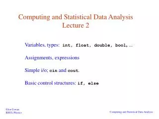
Statistical Methods for Particle Physics Lecture 1: introduction & statistical tests
430 likes | 460 Vues
Explore fundamental statistical concepts, parameter estimation, and statistical tests in particle physics. Learn about multivariate methods, nuisance parameters, and more. Join the lecture to enhance your understanding.

Statistical Methods for Particle Physics Lecture 1: introduction & statistical tests
E N D
Presentation Transcript
Statistical Methods for Particle PhysicsLecture 1: introduction & statistical tests https://indico.cern.ch/event/738002/ IX NExT PhD Workshop: Decoding New Physics Cosener’s House, Abingdon 8-11 July 2019 Glen Cowan Physics Department Royal Holloway, University of London g.cowan@rhul.ac.uk www.pp.rhul.ac.uk/~cowan NExT Workshop, 2019 / GDC Lecture 1 TexPoint fonts used in EMF. Read the TexPoint manual before you delete this box.: AAAA
Outline Lecture 1: Introduction and review of fundamentals Review of probability Parameter estimation, maximum likelihood Statistical tests for discovery and limits Lecture 2: Multivariate methods Neyman-Pearson lemma Fisher discriminant, neural networks Boosted decision trees Lecture 3: Further topics Nuisance parameters (Bayesian and frequentist) Experimental sensitivity Revisiting limits NExT Workshop, 2019 / GDC Lecture 1
Some statistics books, papers, etc. G. Cowan, Statistical Data Analysis, Clarendon, Oxford, 1998 R.J. Barlow, Statistics: A Guide to the Use of Statistical Methods in the Physical Sciences, Wiley, 1989 Ilya Narsky and Frank C. Porter, Statistical Analysis Techniques in Particle Physics, Wiley, 2014. Luca Lista, Statistical Methods for Data Analysis in Particle Physics, Springer, 2017. L. Lyons, Statistics for Nuclear and Particle Physics, CUP, 1986 F. James., Statistical and Computational Methods in Experimental Physics, 2nd ed., World Scientific, 2006 S. Brandt, Statistical and Computational Methods in Data Analysis, Springer, New York, 1998 (with program library on CD) M. Tanabashi et al. (PDG), Phys. Rev. D 98, 030001 (2018); see also pdg.lbl.gov sections on probability, statistics, Monte Carlo NExT Workshop, 2019 / GDC Lecture 1
Theory ↔ Statistics ↔ Experiment Theory (model, hypothesis): Experiment: + data selection + simulation of detector and cuts NExT Workshop, 2019 / GDC Lecture 1
Quick review of probablility NExT Workshop, 2019 / GDC Lecture 1
Frequentist Statistics − general philosophy In frequentist statistics, probabilities are associated only with the data, i.e., outcomes of repeatable observations (shorthand: ). Probability = limiting frequency Probabilities such as P (Nature is supersymmetric), P (0.117 < αs < 0.119), etc. are either 0 or 1, but we don’t know which. The tools of frequentist statistics tell us what to expect, under the assumption of certain probabilities, about hypothetical repeated observations. A hypothesis is is preferred if the data are found in a region of high predicted probability (i.e., where an alternative hypothesis predicts lower probability). NExT Workshop, 2019 / GDC Lecture 1
Bayesian Statistics − general philosophy In Bayesian statistics, use subjective probability for hypotheses: probability of the data assuming hypothesis H (the likelihood) prior probability, i.e., before seeing the data posterior probability, i.e., after seeing the data normalization involves sum over all possible hypotheses Bayes’ theorem has an “if-then” character: If your prior probabilities were π(H), then it says how these probabilities should change in the light of the data. No general prescription for priors (subjective!) NExT Workshop, 2019 / GDC Lecture 1
Distribution, likelihood, model Suppose the outcome of a measurement is x. (e.g., a number of events, a histogram, or some larger set of numbers). The probability density (or mass) function or ‘distribution’ of x, which may depend on parameters θ, is: P(x|θ) (Independent variable is x; θ is a constant.) If we evaluate P(x|θ) with the observed data and regard it as a function of the parameter(s), then this is the likelihood: L(θ) = P(x|θ) (Data x fixed; treat L as function of θ.) We will use the term ‘model’ to refer to the full function P(x|θ) that contains the dependence both on x and θ. NExT Workshop, 2019 / GDC Lecture 1
Quick review of frequentist parameter estimation Suppose we have a pdf characterized by one or more parameters: random variable parameter Suppose we have a sample of observed values: We want to find some function of the data to estimate the parameter(s): ←estimator written with a hat Sometimes we say ‘estimator’ for the function of x1, ..., xn; ‘estimate’ for the value of the estimator with a particular data set. NExT Workshop, 2019 / GDC Lecture 1
Maximum likelihood The most important frequentist method for constructing estimators is to take the value of the parameter(s) that maximize the likelihood: The resulting estimators are functions of the data and thus characterized by a sampling distribution with a given (co)variance: In general they may have a nonzero bias: Under conditions usually satisfied in practice, bias of ML estimators is zero in the large sample limit, and the variance is as small as possible for unbiased estimators. ML estimator may not in some cases be regarded as the optimal trade-off between these criteria (cf. regularized unfolding). NExT Workshop, 2019 / GDC Lecture 1
ML example: parameter of exponential pdf Consider exponential pdf, and suppose we have i.i.d. data, The likelihood function is The value of τ for which L(τ) is maximum also gives the maximum value of its logarithm (the log-likelihood function): NExT Workshop, 2019 / GDC Lecture 1
ML example: parameter of exponential pdf (2) Find its maximum by setting → Monte Carlo test: generate 50 values using t = 1: We find the ML estimate: NExT Workshop, 2019 / GDC Lecture 1
Frequentist statistical tests Consider a hypothesis H0 and alternative H1. A test of H0 is defined by specifying a critical region wof the data space such that there is no more than some (small) probability α, assuming H0 is correct, to observe the data there, i.e., P(x∈ w | H0 ) ≤ α Need inequality if data are discrete. α is called the size or significance level of the test. If x is observed in the critical region, reject H0. data space Ω critical region w NExT Workshop, 2019 / GDC Lecture 1
Definition of a test (2) But in general there are an infinite number of possible critical regions that give the same significance level α. So the choice of the critical region for a test of H0 needs to take into account the alternative hypothesis H1. Roughly speaking, place the critical region where there is a low probability to be found ifH0 is true, but high if H1 is true: NExT Workshop, 2019 / GDC Lecture 1
Type-I, Type-II errors Rejecting the hypothesis H0 when it is true is a Type-I error. The maximum probability for this is the size of the test: P(x∈ W | H0 ) ≤ α But we might also accept H0 when it is false, and an alternative H1 is true. This is called a Type-II error, and occurs with probability P(x∈ S -W | H1 ) = β One minus this is called the power of the test with respect to the alternative H1: Power = 1 -β NExT Workshop, 2019 / GDC Lecture 1
p-values for a set of Suppose hypothesis H predicts pdf observations We observe a single point in this space: What can we say about the validity of H in light of the data? Express level of compatibility by giving the p-value for H: p = probability, under assumption of H, to observe data with equal or lesser compatibility with H relative to the data we got. This is not the probability that H is true! Requires one to say what part of data space constitutes lesser compatibility with H than the observed data (implicitly this means that region gives better agreement with some alternative). NExT Workshop, 2019 / GDC Lecture 1
Test statistics and p-values Consider a parameter μ proportional to rate of signal process. Often construct a test statistic, qμ, which reflects the level of agreement between the data and the hypothesized value μ. For examples of statistics based on the profile likelihood ratio, see, e.g., CCGV, EPJC 71 (2011) 1554; arXiv:1007.1727. Usually define qμ such that higher values represent increasing incompatibility with the data, so that the p-value of μ is: observed value of qμ pdf of qμ assuming μ Equivalent formulation of test: reject μ if pμ < α. NExT Workshop, 2019 / GDC Lecture 1
Confidence interval from inversion of a test Carry out a test of size α for all values of μ. The values that are not rejected constitute a confidence interval for μ at confidence level CL = 1 – α. The confidence interval will by construction contain the true value of μ with probability of at least 1 – α. The interval will cover the true value of μ with probability ≥ 1 - α. Equivalently, the parameter values in the confidence interval have p-values of at least α. To find edge of interval (the “limit”), setpμ = α and solve for μ. NExT Workshop, 2019 / GDC Lecture 1
Significance from p-value Often define significance Z as the number of standard deviations that a Gaussian variable would fluctuate in one direction to give the same p-value. 1 - TMath::Freq TMath::NormQuantile NExT Workshop, 2019 / GDC Lecture 1
The Poisson counting experiment Suppose we do a counting experiment and observe n events. Events could be from signal process or from background – we only count the total number. Poisson model: s = mean (i.e., expected) # of signal events b = mean # of background events Goal is to make inference about s, e.g., test s = 0 (rejecting H0 ≈ “discovery of signal process”) test all non-zero s (values not rejected = confidence interval) In both cases need to ask what is relevant alternative hypothesis. NExT Workshop, 2019 / GDC Lecture 1
Poisson counting experiment: discovery p-value Suppose b = 0.5 (known), and we observe nobs = 5. Should we claim evidence for a new discovery? Give p-value for hypothesis s = 0: NExT Workshop, 2019 / GDC Lecture 1
Poisson counting experiment: discovery significance Equivalent significance for p = 1.7 × 10⁻⁴: Often claim discovery if Z > 5 (p < 2.9 × 10⁻⁷, i.e., a “5-sigma effect”) In fact this tradition should be revisited: p-value intended to quantify probability of a signal-like fluctuation assuming background only; not intended to cover, e.g., hidden systematics, plausibility signal model, compatibility of data with signal, “look-elsewhere effect” (~multiple testing), etc. NExT Workshop, 2019 / GDC Lecture 1
Frequentist upper limit on Poisson parameter Consider again the case of observing n ~ Poisson(s + b). Suppose b = 4.5, nobs = 5. Find upper limit on s at 95% CL. Relevant alternative is s = 0 (critical region at low n) p-value of hypothesized s is P(n ≤ nobs; s, b) Upper limit sup at CL = 1 – α found from NExT Workshop, 2019 / GDC Lecture 1
Frequentist upper limit on Poisson parameter Upper limit sup at CL = 1 – α found from ps = α. nobs = 5, b = 4.5 NExT Workshop, 2019 / GDC Lecture 1
n ~ Poisson(s+b): frequentist upper limit on s For low fluctuation of n formula can give negative result for sup; i.e. confidence interval is empty. NExT Workshop, 2019 / GDC Lecture 1
Large sample distribution of the profile likelihood ratio (Wilks’ theorem, cont.) Suppose problem has likelihood L(θ,ν), with ← parameters of interest ← nuisance parameters Want to test point in θ-space. Define profile likelihood ratio: , where “profiled” values of ν and define qθ = -2 ln λ(θ). Wilks’ theorem says that distribution f (qθ|θ,ν) approaches the chi-square pdf for N degrees of freedom for large sample (and regularity conditions), independent of the nuisance parameters ν. NExT Workshop, 2019 / GDC Lecture 1
p-values in cases with nuisance parameters Suppose we have a statistic qθ that we use to test a hypothesized value of a parameter θ, such that the p-value of θ is Fundamentally we want to reject θ only if pθ < α for all ν. → “exact” confidence interval Recall that for statistics based on the profile likelihood ratio, the distribution f(qθ|θ,ν) becomes independent of the nuisance parameters in the large-sample limit. But in general for finite data samples this is not true; one may be unable to reject some θ values if all values of ν must be considered, even those strongly disfavoured by the data (resulting interval for θ“overcovers”). NExT Workshop, 2019 / GDC Lecture 1
Profile construction (“hybrid resampling”) Approximate procedure is to reject θ if pθ ≤ αwhere the p-value is computed assuming the profiled values of the nuisance parameters: “double hat” notation means value of parameter that maximizes likelihood for the given θ. The resulting confidence interval will have the correct coverage for the points . Elsewhere it may under- or overcover, but this is usually as good as we can do (check with MC if crucial or small sample problem). NExT Workshop, 2019 / GDC Lecture 1
Prototype search analysis Search for signal in a region of phase space; result is histogram of some variable x giving numbers: Assume the ni are Poisson distributed with expectation values strength parameter where background signal NExT Workshop, 2019 / GDC Lecture 1
Prototype analysis (II) Often also have a subsidiary measurement that constrains some of the background and/or shape parameters: Assume the mi are Poisson distributed with expectation values nuisance parameters (θs, θb,btot) Likelihood function is NExT Workshop, 2019 / GDC Lecture 1
The profile likelihood ratio Base significance test on the profile likelihood ratio: maximizes L for specified μ maximize L The likelihood ratio of point hypotheses gives optimum test (Neyman-Pearson lemma). The profile LR hould be near-optimal in present analysis with variable μ and nuisance parameters θ. NExT Workshop, 2019 / GDC Lecture 1
Test statistic for discovery Try to reject background-only (μ= 0) hypothesis using i.e. here only regard upward fluctuation of data as evidence against the background-only hypothesis. Note that even though here physically μ ≥ 0, we allow to be negative. In large sample limit its distribution becomes Gaussian, and this will allow us to write down simple expressions for distributions of our test statistics. NExT Workshop, 2019 / GDC Lecture 1
Cowan, Cranmer, Gross, Vitells, arXiv:1007.1727, EPJC 71 (2011) 1554 Distribution of q0 in large-sample limit Assuming approximations valid in the large sample (asymptotic) limit, we can write down the full distribution of q0 as The special case μ′ = 0 is a “half chi-square” distribution: In large sample limit, f(q0|0) independent of nuisance parameters; f(q0|μ′) depends on nuisance parameters through σ. NExT Workshop, 2019 / GDC Lecture 1
p-value for discovery Large q0 means increasing incompatibility between the data and hypothesis, therefore p-value for an observed q0,obs is use e.g. asymptotic formula From p-value get equivalent significance, NExT Workshop, 2019 / GDC Lecture 1
Cowan, Cranmer, Gross, Vitells, arXiv:1007.1727, EPJC 71 (2011) 1554 Cumulative distribution of q0, significance From the pdf, the cumulative distribution of q0 is found to be The special case μ′ = 0 is The p-value of the μ = 0 hypothesis is Therefore the discovery significance Z is simply NExT Workshop, 2019 / GDC Lecture 1
Cowan, Cranmer, Gross, Vitells, arXiv:1007.1727, EPJC 71 (2011) 1554 Monte Carlo test of asymptotic formula Here take τ = 1. Asymptotic formula is good approximation to 5σ level (q0 = 25) already for b ~ 20. NExT Workshop, 2019 / GDC Lecture 1
Cowan, Cranmer, Gross, Vitells, arXiv:1007.1727, EPJC 71 (2011) 1554 Test statistic for upper limits For purposes of setting an upper limit on μ use where I.e. when setting an upper limit, an upwards fluctuation of the data is not taken to mean incompatibility with the hypothesized μ: From observed qμ find p-value: Large sample approximation: 95% CL upper limit on μ is highest value for which p-value is not less than 0.05. NExT Workshop, 2019 / GDC Lecture 1
Cowan, Cranmer, Gross, Vitells, arXiv:1007.1727, EPJC 71 (2011) 1554 Monte Carlo test of asymptotic formulae Consider again n ~ Poisson (μs + b), m ~ Poisson(τb) Use qμ to find p-value of hypothesized μ values. E.g. f (q1|1) for p-value of μ=1. Typically interested in 95% CL, i.e., p-value threshold = 0.05, i.e., q1 = 2.69 or Z1 = √q1 = 1.64. Median[q1 |0] gives “exclusion sensitivity”. Here asymptotic formulae good for s = 6, b = 9. NExT Workshop, 2019 / GDC Lecture 1
Finishing Lecture 1 So far we have introduced the basic ideas of: Probability (frequentist, subjective) Parameter estimation (maximum likelihood) Statistical tests (reject H if data found in critical region) Confidence intervals (region of parameter space not rejected by a test of each parameter value) We saw tests based on the profile likelihood ratio statistic Sampling distribution independent of nuisance parameters in large sample limit; simple formulae for p-value. Formula for upper limit can give empty confidence interval if e.g. data fluctuate low relative to expected background. More on this later. NExT Workshop, 2019 / GDC Lecture 1
Extra slides NExT Workshop, 2019 / GDC Lecture 1
How to read the p0 plot The “local”p0 means the p-value of the background-only hypothesis obtained from the test of μ = 0 at each individual mH, without any correct for the Look-Elsewhere Effect. The “Expected” (dashed) curve gives the median p0 under assumption of the SM Higgs (μ = 1) at each mH. ATLAS, Phys. Lett. B 716 (2012) 1-29 The blue band gives the width of the distribution (±1σ) of significances under assumption of the SM Higgs. NExT Workshop, 2019 / GDC Lecture 1
How to read the green and yellow limit plots For every value of mH, find the upper limit on μ. Also for each mH, determine the distribution of upper limits μup one would obtain under the hypothesis of μ = 0. The dashed curve is the median μup, and the green (yellow) bands give the ± 1σ (2σ) regions of this distribution. ATLAS, Phys. Lett. B 716 (2012) 1-29 NExT Workshop, 2019 / GDC Lecture 1
How to read the “blue band” On the plot of versus mH, the blue band is defined by i.e., it approximates the 1-sigma error band (68.3% CL conf. int.) ATLAS, Phys. Lett. B 716 (2012) 1-29 NExT Workshop, 2019 / GDC Lecture 1