Download
1 / 39
390 likes | 420 Vues
Discover how to leverage hardware basics like main memory, disk space, and speed to construct efficient inverted indexes for large collections. Explore strategies like hashing and B-trees, and learn how to use the Blocked Sort-Based Indexing (BSBI) method for faster index construction.

E N D
Some Hardware Basics • Access to data in memory is much faster than access to data on disk. • Disk seeks: No data is transferred from disk while the disk head is being positioned. • Therefore: Transferring one large chunk of data from disk to memory is faster than transferring many small chunks. • Disk I/O is block-based: Reading and writing of entire blocks (as opposed to smaller chunks).
Hardware Basics • Servers now typically have tens of GBs of main memory • Available disk space is several (2–3) orders of magnitude larger • Terabyte disks are common • Fault tolerance: It’s much cheaper to use many regular machines rather than one fault tolerant machine. • Access to main memory is much faster than access to disk • seek time is the time for the disk head to move where the data is located • therefore chunks of data are stored contiguously
Recall Earlier Index Construction • Documents are parsed to extract words and these are saved with the Document ID. Doc 1 Doc 2 I did enact Julius Caesar I was killed i' the Capitol; Brutus killed me. So let it be with Caesar. The noble Brutus hath told you Caesar was ambitious
After all documents have been parsed, the inverted file is sorted by terms. Key Step - Sorting We focus on this sort step. We have 100M items to sort.
Scaling Index Construction • In-memory index construction does not scale • Can’t stuff entire collection into memory, sort, then write back • How can we construct an index for very large collections? • Taking into account the hardware constraints we just assumed . . . • Memory, disk, speed, etc.
One Possible StrategyHashing to Hold the Dictionary • Hashing has been used by search engines to maintain the dictionary • Each term is hashed to an integer over a large space so collisions are minimized • Similarly, query terms are hashed and posting lists are returned • Problems: • no easy way to find minor variants, e.g. resume vs. résume hash to very different buckets • no easy way to find all words with a common prefix, e.g. automat*
Another Strategy:B-Trees to Hold the Dictionary • a B-tree is a self-balancing tree data structure that keeps data sorted and allows searches, sequential access, insertions, and deletions in logarithmic time • the B-tree is optimized for systems that read and write large blocks of data and often used for data that does not fit in memory • below is a B-tree of order 5
Recall Some Facts About B-Trees • In B-trees, internal (non-leaf) nodes can have a variable number of child nodes within some pre-defined range. • When data is inserted or removed from a node, the number of child nodes changes. Internal nodes may be joined or split. • B-trees do not need re-balancing as frequently as other self-balancing search trees • The lower and upper bounds on the number of child nodes are typically fixed for a particular implementation. For example, in a 2-3 B-tree, each internal node may have only 2 or 3 child nodes • a B-tree of height h, n entries, and m node size with all its nodes completely filled • has n= mh+1−1 entries • the best case height is: ceil( log m (n + 1) ) - 1 • the worst case height is: <= floor ( log d (n + 1) / 2 )
Using Sorting to Create/Maintain the Dictionary • Why we need to use disk-based sorting to construct the index • To create the inverted index we follow these steps: • Read docs, extract terms and form (term, docID) pairs • Sort the pairs using term as the sort key • Create a posting list for each term, a list of docIDs holding the term • Sort the terms • If there are more terms than can fit in memory, we need an external sorting algorithm • Conclusion: we need to store intermediate results on disk.
Sort Using Disk as “memory”? • Can we use the same index construction algorithm that we used for in-memory index, for larger collections, but by using disk instead of memory? • Answer: • No: an internal sorting algorithm with access to elements converted to disk accesses requires far too many • e.g. sorting T = 100,000,000 records on disk is too slow – too many disk seeks • We need a specially designed external sorting algorithm • an algorithm that attempts to minimize disk accesses • *T stands for tokens or intuitively "words"
Our Book Uses This Example 100,000,000 tokens, 4 bytes for termID, 4 bytes for docID, requires 0.8GBs of storage implying sorting in main memory is insufficient (using the assumptions at the beginning of the lecture)
BSBI: Blocked Sort-Based Indexing (Sorting with fewer disk seeks) • Recall • 12-byte (4+4+4) records (term, doc, freq) • These are generated as we parse docs • Must now sort 100M such 12-byte records by term • Define a Block ~ 10M such records • Can easily fit multiple blocks simultaneously into memory. • For 100M records we will have 10 such blocks to start with. • Basic idea of algorithm: • Accumulate postings until they fill up a block, then sort the block and write it to disk. • Then merge the blocks into one long sorted order
Merging in Block Sort-Based Indexing 2. sort the blocks by terms in memory 1. read two 10M blocks from disk 3. write the results back to disk
Sorting 10 Blocks of 10M Records • First, read each block and sort within: • Quicksort takes 2N ln N expected steps • In our case 2 x (10M ln 10M) steps • Suppose the time to sort is TSort, then • 10 times TSort – gives us 10 sorted runs of 10M records each. • Merge the results into a single, sorted postings list, producing the algorithm on the next slide
Block Sort-Based Indexing Algorithm n is the block number generates (termId,docId) pairs inversion involves two steps: 1. sorting the termID-docID pairs, 2. collect all termID-docID with the same termID into a postings list inverted blocks are stored in files f1to fn; fmerged contains the merged index step 7 is outside the loop; it merges all blocks into one ordered postings list
1 3 2 4 How to Merge the Sorted Runs? • Can do binary merges, with a merge tree of log210 = 4 layers • called a binary merge step • During each layer, read into memory runs in blocks of 10M, merge, write back. • Open all block files simultaneously and maintain small read buffers for the blocks we are reading and a write buffer for the final merged index 2 1 Merged run. 3 4 Runs being merged. Disk
Sec. 4.2 How to Merge the Sorted Runs? • Computing time for BSBI is O(T log T) as the sorting step takes the longest time • Instead of doing a 2-way merge, it is more efficient to do a multi-way merge, where you are reading from all blocks simultaneously • Providing you read decent-sized chunks of each block into memory and then write out a decent-sized output chunk, then you’re not killed by disk seeks
Sec. 4.3 Remaining Problem with Sort-Based Algorithm • Our assumption was: we can keep the dictionary in memory • We need the dictionary (which grows dynamically) in order to implement a term to termID mapping. • Actually, we could work with term, docID postings instead of termID, docID postings however. . . • . . . but then intermediate files become very large. (We would end up with a scalable, but very slow index construction method)
Sec. 4.3 SPIMI: Single-Pass In-Memory Indexing • Problem: blocked sort-based indexing scales well, but it needs a data structure for mapping terms to termIDs • Solution idea 1: Generate separate dictionaries for each block – no need to maintain term-termID mapping across blocks. • Solution idea 2: Don’t sort at all. Accumulate postings in postings lists as they occur. • With these two ideas we can generate a complete inverted index for each block without needing to sort it; • These separate indexes can then be merged into one big index.
Sec. 4.3 Single Pass InMemoryIndexing-Invert Notes: - is called repeatedly on the token stream - uses terms instead of termIDs - writes each block's dictionary to disk - either starts a new dictionary for the next block - a term occurs for the first time, else - posting list for existing term is returned dictionary is initially empty • Merging of blocks is analogous to Block Sort-Based Indexing • No sorting is required and each posting list is immediately available generate (term,docId) output_file contains the final inverted index
Sec. 4.3 SPIMI: Compression • Time complexity of SPIMI is O(T) as all operations are linear in the size of the collection • Compression will make SPIMI even more efficient. • Compression of terms • Compression of postings
Sec. 4.5 Dynamic Indexing • Up to now, we have assumed that collections are static • They rarely are: • Documents come in over time and need to be inserted. • Documents are deleted and modified. • This means that the dictionary and postings lists have to be continually modified: • Postings updates for terms already in dictionary • New terms added to dictionary
Sec. 4.5 Simplest Approach • Maintain “big” main index • New docs go into “small” auxiliary index • Search across both; merge results periodically • Deletions • Initially create an invalidation bit-vector for deleted docs • Filter docs output on a search result by this invalidation bit-vector, so deleted docs are not returned as results; • Periodically, re-index into one main index
Sec. 4.5 Issues with Main and Auxiliary Indexes • Each time the auxiliary list gets large, merge it into the main index; • Problem: you may have frequent merges • Poor performance during merge • Actually: • Merging of the auxiliary index into the main index is efficient if we keep a separate file for each postings list • Merge is the same as a simple append • But then we would need a lot of files – inefficient for OS
Sec. 4.5 Logarithmic Merge(see accompanying video) • Maintain a series of indexes, each twice as large as the previous one • At any time, some of these powers of 2 are instantiated • Keep smallest index (Z0) in memory; • this is the smallest auxiliary postings list • Larger ones (I0, I1, …) are kept on disk • If Z0 gets too big (> n), write to disk as I0 or merge with I0 (if I0 already exists) creating Z1 • Either write merge Z1 to disk as I1 (if no I1 exists) or merge with I1 to form Z2
Sec. 4.5 Logarithmic Merging Each token (termID, docID) is initially added to in-memory index Z0 by LMergeAddToken. LogarithmicMerge initializes Z0 and indexes
Sec. 4.5 Logarithmic Merge • Auxiliary and main index: index construction time is O(T2) as each posting is touched in each merge. • Logarithmic merge: Each posting is merged O(log T) times, so complexity is O(T log T) • So logarithmic merge is much more efficient for index construction • But query processing now requires the merging of O(log T) indexes • Whereas it is O(1) if you just have a main and auxiliary index
Sec. 4.4 Distributed Indexing • Note: the BSBI and SPIMI algorithms assume that the data collection is static • For web-scale indexing: • cannot use a single machine • must use a distributed computing cluster • Besides, individual machines are fault-prone • Can unpredictably slow down or fail • How do we exploit such a pool of machines? BSBI-Block Sort-Based Indexing; SPIMI-Single Pass In_Memory Indexing
Sec. 4.4 Web Search Engine Data Centers • Web search data centers (Google, Bing, Baidu) mainly contain commodity machines. • Estimate: both Google and Bing are reporting the use of more than 1 million servers • Notes: J. Pearn estimates Google at 1,700,000 servers as of Jan. 2012, https://plus.google.com/+JamesPearn/posts/VaQu9sNxJuY • Google data centers are distributed around the world.
Google Data Centers https://www.google.com/about/datacenters/inside/locations/index.html See also the 5 minute video at: https://www.google.com/about/datacenters/inside/
Sec. 4.4 Distributed Indexing • As the web is so large, search engines use computer clusters to hold the index • Therefore they need to develop distributed indexing algorithms for insertion of data and for processing queries • Commonly each node contains the index for a subset of documents (document partitioning) • Each query is distributed to all nodes • the top k results from each node are merged to produce the final result • However, we begin with a term partitioned index
Sec. 4.4 Term Partitioned Indexing Using Map/Reduce • General strategy • Divide the work into chunks • Assign chunks to machines • expect machines to fail, and handle re-assignment • Maintain a master machine directing the indexing job – considered “safe” • Master machine assigns each task to an idle machine from a pool. • Machines will either be solving two sets of parallel tasks • Parsers • Inverters • Each split is a subset of documents (corresponding to blocks in BSBI/SPIMI) • (Block Sort-Based Indexing/Single Pass In-Memory Indexing)
Sec. 4.4 Parsers • Master assigns a split to an idle parser machine • Parser reads a document at a time and emits (term, doc) pairs • Parser writes pairs into j partitions • Each partition is for a range of terms’ first letters • (e.g., a-f, g-p, q-z) – here j = 3
Sec. 4.4 Inverters • An inverter collects all (term,doc) pairs (= postings) for one term-partition. • Sorts and writes to postings lists
Sec. 4.4 Data flow Master assign assign Postings Parser Inverter a-f g-p q-z a-f Parser a-f g-p q-z Inverter g-p Inverter splits q-z Parser a-f g-p q-z Map phase Reduce phase Segment files
Sec. 4.4 Map/Reduce • The index construction algorithm we just described is an instance of MapReduce. • MapReduce (Dean and Ghemawat 2004) is a robust and conceptually simple framework for distributed computing … • … without having to write code for the distribution part. • They describe the Google indexing system (ca. 2002) as consisting of a number of phases, each implemented in MapReduce.
Sec. 4.4 MapReduce • Index construction was just one phase. • Another phase: transforming a term-partitioned index into a document-partitioned index. • Term-partitioned: one machine handles a subrange of terms • Document-partitioned: one machine handles a subrange of documents • Most search engines use a document-partitioned index … better load balancing, etc.
Sec. 4.4 Schema for Index Construction in MapReduce • Schema of map and reduce functions • map: input → list(k, v) • reduce: (k,list(v)) → output where k stands for key and v stands for value; key/value pairs are reduced to (key, list of values) • Instantiation of the schema for index construction • map: collection → list(termID, docID) • reduce: (<termID1, list(docID)>, <termID2, list(docID)>, …) → (postings list1, postings list2, …)