Download
1 / 64
650 likes | 829 Vues
V.3 Top-k Query Processing. 3.1 IR-style heuristics for efficient inverted index scans 3.2 Fagin’s family of threshold algorithms (TA) 3.3 Approximation algorithms based on TA. Indexing with Score-ordered Lists. Documents: d 1 , …, d n. Index-list entries stored in descending order of

E N D
V.3 Top-k Query Processing 3.1 IR-style heuristics for efficient inverted index scans 3.2 Fagin’s family of threshold algorithms (TA) 3.3 Approximation algorithms based on TA IR&DM, WS'11/12
Indexing with Score-ordered Lists Documents:d1, …, dn Index-list entries stored in descending order of per-term score (impact-ordered lists). d10 s(t1,d1) = 0.9 … s(tm,d1) = 0.2 sort Aims to avoid having to read entire lists: → rather scan only (short) prefixes of lists for the top-ranked answers. Index lists d78 0.9 d23 0.8 d10 0.8 d1 0.7 d88 0.2 t1 … d64 0.8 d23 0.6 d10 0.6 d10 0.2 d78 0.1 t2 … d10 0.7 d78 0.5 d64 0.4 d99 0.2 d34 0.1 t3 … IR&DM, WS'11/12
Query Processing on Score-ordered Lists Top-k aggregation query over R(docId, A1, ..., Am) partitions: Select docId, score(R1.A1, ..., Rm.Am)As Aggr From Outer Join R1, …, Rm Order By AggrDescLimit k with monotone score aggregation function score: score: Rm→ R, s.t. ( xi xi’ ) score(x1…xm) score(x1’…xm’) • Precompute index lists in descending attr-value order • (score-ordered, impact-ordered). • Scan lists by sorted access(SA) in round-robin manner. • Perform random accesses (RA) by docId when convenient. • Compute aggregation score incrementallyin candidate queue. • Compute score bounds for candidate results and • stop when threshold test guarantees correct top-k • (or when heuristics indicate “good enough” approximation). IR&DM, WS'11/12
V.3.1 Heuristic Top-k Algorithms • General pruning and index-access ordering heuristics: • Disregard index lists with low idf(below given threshold). • For scheduling index scans, give priority to index lists • that are short and have high idf. • Stop adding candidates to the queue if we run out of memory. • Stop scanning a particular list if the local scores in it become low. • … IR&DM, WS'11/12
List L1 List L2 List L3 Buckley’85 [Buckley & Lewit: SIGIR’85] Top-1: d83 0.9 Upper: dvirt 2.2 Top-1: d17 1.4 Upper: dvirt 1.8 Top-1: d17 1.4 Upper: dvirt 1.3 lists sorted by desc. local score (e.g., tf*idf) Note: this is a simplified version of Buckley’s original algorithm, which considers an upper bound for the actual (k+1)-ranked document instead of the virtual document. If this (k+1)-ranked document is computed properly (e.g., all candidates are kept and updated in a queue), then this is the first correct top-k algorithm based on sequential data access proposed in the literature! IR&DM, WS'11/12 Incrementally scan lists Li in round-robin fashion. For each access, aggregate local score to corresponding document’s global score. The sum of local scores at the current scan positions is an upper bound for all unseen documents (“virtual doc”). Stop if this upper bound is less than current k-th best document’s partial score.
Quit & Continue [Moffat/Zobel: TOIS’96] Focus on scoring of the form with Implementation is based on a hash array of accumulators for summing up the partial scores of candidate results. • quit heuristics: (with lists ordered by tf or tf*idl): • Ignore index list Li if idf(ti) is below threshold. • Stop scanning Liif tf(ti,dj)*idf(ti)*idl(dj) drops below threshold. • Stop scanning Li when the number of accumulators is too high. continue heuristics: Upon reaching threshold, continue scanning index lists and aggregate scores but do not add any new documents to the accumulators. IR&DM, WS'11/12
Greedy Index Access Scheduling (I) Assume index lists are sorted by descending si(ti,dj) (e.g., using tf(ti,dj) or tf(ti,dj)*idl(dj) values): Open scan cursors on all m index lists L(i); Repeat Find pos(g) among current cursor positions pos(i) (i=1..m) with the largest value of si(ti, pos(i)); Update the accumulator of the corresponding doc at pos(g); Increment pos(g); Until stopping condition holds; IR&DM, WS'11/12
Greedy Index Access Scheduling (II)[Güntzer, Balke, Kießling: “Stream-Combine”, ITCC’01] Assume index lists are sorted by descending si(ti,dj): Open scan cursors on all m index lists L(i); Repeat For sliding window w (e.g., 100 steps), find pos(g) among current cursor positions pos(i) (i=1..m) with the largest gradient (si(ti, pos(i)–w) – si(ti, pos(i)))/w; Update the accumulator of the corresponding doc at pos(g); Increment pos(g); Until stopping condition holds; IR&DM, WS'11/12
QP with Authority/Similarity Scoring [Long/Suel: VLDB’03] Focus on score(q,dj) = r(dj) + s(q,dj) with normalization r() a, s() b (and often a+b=1) Keep index lists sorted in descending order of “static” authority r(dj) Conservative authority-based pruning: high(0) := max{r(pos(i)) | i=1..m}; high := high(0) + b; high(i) := r(pos(i)) + b; Stop scanning i-th index list when high(i) < min score of top-k; Terminate when high < min score of top-k; → Effective when total score of top-k results is dominated by r First-k’ heuristics: Scan all m index lists until k’ k docs have been found that appear in all lists. → This stopping condition is easy to check because lists are sorted by r. IR&DM, WS'11/12
Top-k with “Champion Lists” Idea (Brin/Page’98): In addition to the full index lists Li sorted by r, keep short “champion lists”(aka. “fancy lists”) Fi that contain docs djwith the highest values of si(ti,dj)and sort these lists by r. Champions First-k’ heuristics: Compute total score for all docs in Fi (i=1..m) and keep top-k results; Cand := iFi iFi; For each dj Cand do {compute partial score of dj}; Scan full index lists Li (i=1..k); if pos(i) Cand {add si(ti,pos(i)) to partial score of doc at pos(i)} else {add pos(i) to Cand and set its partial score to si(ti,pos(i))}; Terminate the scan when we have k’ docs with complete total score; IR&DM, WS'11/12
V.3.2 Fagin’s Family of Threshold Algorithms • Different variants of TA family have been developed by several groups at around the same time. • Solid theoretical foundation (including proofs of instance optimality) provided in: • [R. Fagin, A. Lotem, M. Naor: Optimal Aggregation Algorithms for Middleware, JCSS’03] • Implementation (e.g., queue management) not specifiedby Fagin’s framework (but does matter a lot in practice). • Many extensions for approximate variants of TA. IR&DM, WS'11/12 Threshold Algorithm (TA) Original version, often used as synonym for entire family of top-k algorithms. But: eager random access to candidate objects required. Worst-case memory consumption is strictly bounded → O(k) No-Random-Access Algorithm (NRA) No random access required at all, but may have to scan large parts of the index lists. Worst-case memory consumption bounded by index size → O(m*n + k) Combined Algorithm (CA) Cost-model for scheduling well-targeted random accesses to candidate objects. Algorithmic skeleton very similar to NRA, but typically terminates much faster. Worst-case memory consumption bounded by index size → O(m*n + k)
Rank Doc Score Rank Doc Score Rank Doc Score 1 d10 2.1 1 d10 2.1 1 d10 2.1 Rank Doc Score 2 d78 1.5 2 d78 1.5 2 d78 1.5 1 d10 2.1 2 d64 0.9 1 d78 1.5 2 d64 1.2 1 d78 1.5 2 d78 1.5 Threshold Algorithm (TA) [Fagin’01, Güntzer’00, Nepal’99, Buckley’85] Threshold algorithm (TA): scan index lists; consider d at posi in Li; highi := s(ti,d); if d top-k then { look up s(d) in all lists L with i; score(d) := aggr {s(d) | =1..m}; if score(d) > min-k then add d to top-k and remove min-score d’; min-k := min{score(d’) | d’ top-k}; threshold := aggr {high | =1..m}; if thresholdmin-k then exit; Simple & DB-style; needs only O(k) memory Documents:d1, …, dn d1 s(t1,d1) = 0.7 … s(tm,d1) = 0.2 Query: q = (t1, t2, t3) Index lists k = 2 Rank Doc Score d78 0.9 d23 0.8 d10 0.8 d1 0.7 d88 0.2 t1 Scan depth 1 … Scan depth 2 Scan depth 3 Scan depth 4 1 d78 0.9 d64 0.9 d23 0.6 d10 0.6 d12 0.2 d78 0.1 t2 … 2 d64 0.9 d10 0.7 d78 0.5 d64 0.3 d99 0.2 d34 0.1 t3 … STOP! IR&DM, WS'11/12
No-Random-Access Algorithm (NRA) [Fagin’01, Güntzer’01] No-Random-Access algorithm (NRA): scan index lists; consider d at posi in Li; E(d) := E(d) {i}; highi := s(ti,d); worstscore(d) := aggr{s(t,d) | E(d)}; bestscore(d) := aggr{worstscore(d), aggr{high | E(d)}}; if worstscore(d) > min-k then add d to top-k min-k := min{worstscore(d’) | d’ top-k}; else if bestscore(d) > min-k then cand := cand {d}; threshold := max {bestscore(d’) | d’ cand}; if threshold min-k then exit; Sequential access (SA) faster than random access (RA) Documents:d1, …, dn d1 s(t1,d1) = 0.7 … s(tm,d1) = 0.2 Query: q = (t1, t2, t3) Index lists k = 1 d78 0.9 d23 0.8 d10 0.8 d1 0.7 d88 0.2 t1 Scan depth 1 … Scan depth 2 Scan depth 3 d64 0.8 d23 0.6 d10 0.6 d12 0.2 d78 0.1 t2 … d10 0.7 d78 0.5 d64 0.4 d99 0.2 d34 0.1 t3 … STOP! IR&DM, WS'11/12
Combined Algorithm(CA) [Fagin et al. ‘03] Balanced SA/RA Scheduling: Define cost ratio CRA/CSA =: r (e.g., based on statistics for execution environment (“middleware”), typical values: CRA /CSA ~ 20-10,000 for a hard-disk) Perform NRA (using sorted access only) ... After every r rounds of SA (i.e., after m*r SA steps) perform one RA to look up the unknown scores of the best candidate d(w.r.twortscore(d)) that is not among the current top-k items. Cost competitivenessw.r.t. “optimal schedule” (scan until ihighi ≤ min{bestscore(d) | d final top-k}, then perform RAs for all d’ with bestscore(d’) > min-k): 4m + k IR&DM, WS'11/12
CA Scheduling Example CA: compute top-1 result using one RA after every round of SA L1 L2 L3 A: 0.8 G: 0.7 Y: 0.9 B: 0.2 H: 0.5 A: 0.7 K: 0.19 R: 0.5 P: 0.3 F: 0.17 Y: 0.5 F: 0.25 M: 0.16 W: 0.3 S: 0.25 Z: 0.15 D: 0.25 T: 0.2 W: 0.1 W: 0.2 Q: 0.15 Q: 0.07 A: 0.2 X: 0.1 ... ... ... IR&DM, WS'11/12
CA Scheduling Example L1 L2 L3 A: 0.8 G: 0.7 Y: 0.9 B: 0.2 H: 0.5 A: 0.7 1st round of SA: Y is top-1 w.r.t. worstscore. A is best candidate w.r.t. worstscore. → Schedule RA for all of A’s missing scores. K: 0.19 R: 0.5 P: 0.3 F: 0.17 Y: 0.5 F: 0.25 M: 0.16 W: 0.3 S: 0.25 Z: 0.15 D: 0.25 T: 0.2 W: 0.1 W: 0.2 Q: 0.15 Q: 0.07 A: 0.2 X: 0.1 ... ... ... A: [0.8, 2.4] Y: [0.9, 2.4] candidates: G: [0.7, 2.4] ?: [0.0, 2.4] IR&DM, WS'11/12
CA Scheduling Example L1 L2 L3 A: 0.8 G: 0.7 Y: 0.9 B: 0.2 H: 0.5 A: 0.7 1st round of SA: Y is top-1 w.r.t. worstscore. A is best candidate w.r.t. worstscore. → Schedule RA for all of A’s missing scores. K: 0.19 R: 0.5 P: 0.3 F: 0.17 Y: 0.5 F: 0.25 M: 0.16 W: 0.3 S: 0.25 Z: 0.15 D: 0.25 T: 0.2 W: 0.1 W: 0.2 Q: 0.15 Q: 0.07 A: 0.2 X: 0.1 ... ... ... A: [1.7, 1.7] Y: [0.9, 2.4] candidates: G: [0.7, 2.4] ?: [0.0, 2.4] IR&DM, WS'11/12
CA Scheduling Example execution costs: 6 SA + 1 RA L1 L2 L3 A: 0.8 G: 0.7 Y: 0.9 B: 0.2 H: 0.5 A: 0.7 1st round of SA: Y is top-1 w.r.t. worstscore. A is best candidate w.r.t. worstscore. → Schedule RA for all of A’s missing scores. 2nd round of SA: A is top-1 (worst- and bestscore have converged). All candidate’s (incl. virtual doc) bestscores are below A’s worstscore. → Done! K: 0.19 R: 0.5 P: 0.3 F: 0.17 Y: 0.5 F: 0.25 M: 0.16 W: 0.3 S: 0.25 Z: 0.15 D: 0.25 T: 0.2 W: 0.1 W: 0.2 Q: 0.15 Q: 0.07 A: 0.2 X: 0.1 ... ... ... A: [1.7, 1.7] Y: [0.9, 1.6] candidates: G: [0.7, 1.6] ?: [0.0, 1.4] IR&DM, WS'11/12
A note on counting SA’s vs. RA’s: Although A is looked up in both L2 and L3 via random access in the previous example, this step is typically counted as just a single RA (as this can be implemented by one index lookup over a corresponding index structure that points to all the per-term scores of a document). For SA’s, we count each lookup of a document in one of the index lists as a separate SA. That is, one iteration of SA’s over m lists in round-robin fashion yields m SA’s. Overall, counting the cost of SA’s vs. RA’s is highly implementation-dependent and can also be reflected in the CRA/CSA cost ratio considered by some of these algorithms. For simplicity, we will use the convention above. IR&DM, WS'11/12
TA / NRA / CA Instance Optimality [Fagin et al.’03] Definition: For class A of algorithms and class D of datasets, algorithm B A is instance optimal over A and D if for every AA and DD : cost(B,D) c*O(cost(A,D)) + c’ ( competitiveness c). • Theorem: • TA is instance optimal over all top-k algorithms based on • sorted and random accesses to m lists (no “wild guesses”) • and given cost ratio CRA /CSA. • NRA is instance optimal over all algorithms with SA only. • CA is instance optimal over all algorithms with SA and RA • and given cost ratio CRA /CSA. if “wild guesses” are allowed, then no deterministic algorithm is instance-optimal IR&DM, WS'11/12
Top-k with Boolean Search Conditions • Combination of AND andANDish: (t1 AND … AND tj) tj+1 tj+2… tm • TA family applicable with mandatory probing in AND lists • RA scheduling • (worstscore, bestscore) bookkeeping and pruning • more effective with “boosting weights” for AND lists Combination of AND, “andish”, and NOT: NOT terms considered k.o. criteria for results TA family applicable with mandatory probing for AND and NOT RA scheduling for “expensive predicates” • Combination of AND, OR, NOT in Boolean sense: • Best processed by index lists in docId order (not top-k!) • Construct operator tree and push selective operators down; • needs good query optimizer (selectivity estimation) IR&DM, WS'11/12
Implementation Issues for TA Family • Limitation of asymptotic complexity: • m (#lists) and k (#results) are important parameters • Priority queues: • Straightforward use of a heap (even for Fibonacci) has high overhead • Better: periodic rebuild of queue with partial sort O(n log k) • Memory management: • Peak memory use as important for performance as scan depth • Aim for early candidate pruning even if scan depth stays the same • Hybrid block index: • Pack index entries into big blocks in descending score order • Keep blocks in score order • Keep entries within a block in docId order • After each block read: merge-join first, then PQ update IR&DM, WS'11/12
V.3.3 Approximation Algorithms based on TA • IR heuristicsfor impact-ordered lists [Anh/Moffat: SIGIR’01]: • Accumulator limiting, accumulator thresholding, etc. • Approximation TA [Fagin et al.: JCSS’03]: • -approximation(approx. top-k results)T’ for query q • with > 1 is a set T’ of docs with: • |T’|=k and • For each d’T’ and each d’’T’: *score(q,d’) score(q,d’’) • Modified TA: • ... stop when: min-k aggr (high1, ..., highm) / • Probabilistic Top-k [Theobald et al.: VLDB’04]: • Guarantee only small deviation from exact top-k result • with high probability! IR&DM, WS'11/12
Top-k with Probabilistic Guarantees[M. Theobald et al.: VLDB’04] • Let E(d) denote the query dimensions at which d is evaluated, and let highi be the • high score at the current scan position. • TA family of algorithms is based on following invariant (using sum as aggr.): worstscore(d) bestscore(d) score • Add d to top-k result, if worstscore(d) > min-k. • Drop d only if bestscore(d) ≤ min-k, otherwise keep in • candidate queue. • Often overly conservative in pruning, thus resulting in very long scans of the index lists • (esp. for NRA)! ? Can we drop d from the candidate queue earlier? bestscore(d) min-k worstscore(d) scan depth IR&DM, WS'11/12
Probabilistic Threshold Test[M. Theobald et al.: VLDB’04] • Instead of using exact highi bounds, use RV’s Si to estimate the probability that • d will exceed a certain score mass in its remaining lists: with = min-k at current scan position Probabilistic threshold test: Drop candidate d from queue if p(d) Probabilistic guarantee: (for precision/recall@k) Binomial distribution of true (r) and false (k-r) top-k answers, using ε as upper bound for the probability of missing a true top-k result: E[precision@k] = E[recall@k] = 1 IR&DM, WS'11/12
Convolution f2(x), f3(x) f2(x) δ(d) 2 0 0 1 high2 f3(x) 0 1 high3 Probabilistic Score Predicator Candidate d with 2 E(d), 3 E(d) • Postulating Uniform or Pareto score distribution in [0, highi] • Compute convolution using moment-generating function • Use Chernoff-Hoeffding tail bounds (see Chapter I.1) or • generalized bounds for correlated dimensions (Siegel 1995) • Fitting Poissondistribution or Poisson mixture • Over equidistant values: • Easy and exact convolution! • Score distribution approximated by histograms: • Precomputed for each dimension (e.g. equi-width with n cells 0..n-1) • Pair-wise convolution at query-execution time (producing 2n cells 0..2n-1) IR&DM, WS'11/12
Flexible Scheduling of SA’s and RA’s • Goals: • Decrease highi upper-bounds quickly • Decreases bestscore for candidates • Reduces candidate set • Reduce worstscore-bestscore gap for most promising candidates • Increases min-k threshold • More effective threshold test for other candidates • Ideas (again, heuristics) for better scheduling: • Non-uniform choice of SA steps in different lists • Careful choice of postponed RA steps for promising candidates • when worstscore is high and worstscore-bestscore gap is small IR&DM, WS'11/12
= 1.48 = 1.7 + carefully chosen RAs: score lookups for “interesting” candidates batch of b = i=1..m bi steps: choose bi values so as to achieve high score reduction Advanced Scheduling Example L1 L2 L3 A: 0.8 G: 0.7 Y: 0.9 B: 0.2 H: 0.5 A: 0.7 K: 0.19 R: 0.5 P: 0.3 F: 0.17 Y: 0.5 F: 0.25 M: 0.16 W: 0.3 S: 0.25 Z: 0.15 D: 0.25 T: 0.2 W: 0.1 W: 0.2 Q: 0.15 Q: 0.07 A: 0.2 X: 0.1 ... ... ... IR&DM, WS'11/12
compute top-1 result using flexible SAs and RAs Advanced Scheduling Example L1 L2 L3 A: 0.8 G: 0.7 Y: 0.9 B: 0.2 H: 0.5 A: 0.7 K: 0.19 R: 0.5 P: 0.3 F: 0.17 Y: 0.5 F: 0.25 M: 0.16 W: 0.3 S: 0.25 Z: 0.15 D: 0.25 T: 0.2 W: 0.1 W: 0.2 Q: 0.15 Q: 0.07 A: 0.2 X: 0.1 ... ... ... IR&DM, WS'11/12
Advanced Scheduling Example L1 L2 L3 A: 0.8 G: 0.7 Y: 0.9 B: 0.2 H: 0.5 A: 0.7 K: 0.19 R: 0.5 P: 0.3 F: 0.17 Y: 0.5 F: 0.25 M: 0.16 W: 0.3 S: 0.25 Z: 0.15 D: 0.25 T: 0.2 W: 0.1 W: 0.2 Q: 0.15 Q: 0.07 A: 0.2 X: 0.1 ... ... ... A: [0.8, 2.4] Y: [0.9, 2.4] candidates: G: [0.7, 2.4] ?: [0.0, 2.4] IR&DM, WS'11/12
Advanced Scheduling Example L1 L2 L3 A: 0.8 G: 0.7 Y: 0.9 B: 0.2 H: 0.5 A: 0.7 K: 0.19 R: 0.5 P: 0.3 F: 0.17 Y: 0.5 F: 0.25 M: 0.16 W: 0.3 S: 0.25 Z: 0.15 D: 0.25 T: 0.2 W: 0.1 W: 0.2 Q: 0.15 Q: 0.07 A: 0.2 X: 0.1 ... ... ... A: [1.5, 2.0] Y: [0.9, 1.6] candidates: G: [0.7, 1.6] ?: [0.0, 1.4] IR&DM, WS'11/12
Advanced Scheduling Example L1 L2 L3 A: 0.8 G: 0.7 Y: 0.9 B: 0.2 H: 0.5 A: 0.7 K: 0.19 R: 0.5 P: 0.3 F: 0.17 Y: 0.5 F: 0.25 M: 0.16 W: 0.3 S: 0.25 Z: 0.15 D: 0.25 T: 0.2 W: 0.1 W: 0.2 Q: 0.15 Q: 0.07 A: 0.2 X: 0.1 ... ... ... A: [1.5, 2.0] Y: [1.4, 1.6] candidates: G: [0.7, 1.2] IR&DM, WS'11/12
IO-Top-k: Index-Access Optimized Top-k [Bast et al.: VLDB’06] For SA scheduling plan next b1, ..., bm index scan steps for batch of b steps overall s.t. i=1..m bi = b and benefit(b1, ..., bm) is max! → Solve Knapsack-style NP-hard problem for small batches of scans, or use greedy heuristics for larger batches. Perform additional RAs when helpful: 1) To increase min-k (increase worstscore of d top-k), or 2) to prune candidates (decrease bestscore of d among candidates). Last Probing (2-Phase Schedule): Perform RAs for all candidates when cost of remaining RAs ≤ (estimated) cost of remaining SAs with score-prediction & cost model for deciding RA order. IR&DM, WS'11/12
List 2 List 1 List 3 Algorithm NRA Fagin’s NRA Algorithm: lists sorted by score IR&DM, WS'11/12
current score best-score List 2 List 1 List 3 Algorithm NRA round 1 read one doc from every list Candidates min top-2 score: 0.6 maximum score for unseen docs: 2.1 lists sorted by score min-top-2 < best-score of candidates IR&DM, WS'11/12
List 2 List 1 List 3 Algorithm NRA round 2 read one doc from every list Candidates min top-2 score: 0.9 maximum score for unseen docs: 1.8 lists sorted by score min-top-2 < best-score of candidates IR&DM, WS'11/12
List 2 List 1 List 3 Algorithm NRA round 3 read one doc from every list Candidates min top-2 score: 1.3 maximum score for unseen docs: 1.3 lists sorted by score min-top-2 < best-score of candidates no more new docs can get into top-2 but, extra candidates left in queue IR&DM, WS'11/12
List 2 List 1 List 3 Algorithm NRA round 4 read one doc from every list Candidates min top-2 score: 1.3 maximum score for unseen docs: 1.1 lists sorted by score min-top-2 < best-score of candidates no more new docs can get into top-2 but, extra candidates left in queue IR&DM, WS'11/12
List 2 List 1 List 3 Algorithm NRA round 5 read one doc from every list Candidates min top-2 score: 1.6 maximum score for unseen docs: 0.8 lists sorted by score no extra candidate in queue Done! IR&DM, WS'11/12
List 2 List 1 List 3 Algorithm IO-Top-k Round 1: same as NRA not necessarily round robin Candidates min top-2 score: 0.6 maximum score for unseen docs: 2.1 lists sorted by score min-top-2 < best-score of candidates IR&DM, WS'11/12
List 2 List 1 List 3 Algorithm IO-Top-k Round 2 not necessarily round robin Candidates min top-2 score: 0.9 maximum score for unseen docs: 1.4 lists sorted by score min-top-2 < best-score of candidates IR&DM, WS'11/12
List 2 List 1 List 3 Algorithm IO-Top-k Round 3 not necessarily round robin Candidates min top-2 score: 1.3 maximum score for unseen docs: 1.1 lists sorted by score min-top-2 < best-score of candidates potential candidate for top-2 IR&DM, WS'11/12
List 2 List 1 List 3 Algorithm IO-Top-k Round 4: random access for doc 83 not necessarily round robin Candidates min top-2 score: 1.6 maximum score for unseen docs: 1.1 lists sorted by score no extra candidate in queue random access for doc 83 Done! → fewer sorted accesses → carefully scheduled random access IR&DM, WS'11/12
alchemist magician primadonna director artist wizard investigator intellectual Related (0.48) researcher professor Hyponym (0.749) lecturer: 0.7 scientist scholar lecturer mentor 37: 0.9 92: 0.9 academic, academician, faculty member teacher 67: 0.9 44: 0.8 52: 0.9 22: 0.7 44: 0.8 23: 0.6 55: 0.8 51: 0.6 ... 52: 0.6 ... Query Expansion with Incremental Merging [Theobald et al.: SIGIR’05] Expanded query q: ~“professor” research with expansions exp(ti)={cij | sim(ti,cij) , tiq} based on ontological similarity modulating monotonic score aggregation, e.g., using weighted sum over sim(ti,cij)*s(cij,dl). Incrementally merge index lists instead of computing full expansion! Meta-Index (Ontology / Thesaurus) B+ tree index on terms scholar: 0.6 professor ~professor research 57: 0.6 12: 0.9 lecturer: 0.7 scholar: 0.6 academic: 0.53 scientist: 0.5 ... 44: 0.4 44: 0.4 14: 0.8 52: 0.4 28: 0.6 33: 0.3 17: 0.55 75: 0.3 61: 0.5 ... 44: 0.5 ... → efficient, robust, self-tuning IR&DM, WS'11/12
Query Expansion with Incremental Merging [Theobald et al.: SIGIR 2005] • Principles of the algorithm: • Organize possible expansions exp(t)={cj | sim(t,cj) , tq} • in priority queues based on sim(t,cj) for each t. • For a given q = {t1, tm} do: • Keep track of active expansions for each ti: • actExp(ti) = {ci1, ci2, ...cij} • Scan index lists Lij maintaining cursors pos(Lij) • and score bounds high(Lij) for each list. • At each scan step and for each ti do: • Advance cursor of Lijfor cij actExp(ti) for which • best := high(Lij)*sim(ti,cij) is largest among all of exp(ti) • or add next largest cij’ to actExp(ti) if high(Lij’)*sim(ti,cij’) > best • and proceed in this new list. IR&DM, WS'11/12
c1 d78 0.9 d23 0.8 d10 0.8 d1 0.4 d88 0.3 ... c2 d10 0.7 d64 0.8 d23 0.8 d12 0.2 d78 0.1 ... 0.4 0.72 0.18 c3 d11 0.9 d78 0.9 d64 0.7 d99 0.7 d34 0.6 ... 0.45 0.35 0.9 ~t Incremental-Merge Operator Index list meta data (e.g., histograms) Relevance feedback, thesaurus lookups,… Index list high scores Expansion terms exp(t) = {c1,c2,c3} sim(t, c1 ) = 1.0 Correlation measures, co-occurrence statistics, ontological similarities, … sim(t, c2 ) = 0.9 Expansion similarities • Incremental-merge operator iteratively • called by top-level top-k operator • Sorted Access“getNext()” • in descending order of combined score • sim(ti,cij)*s(cij, dl) sim(t, c3 ) = 0.5 d88 0.3 d78 0.9 d23 0.8 d10 0.8 d64 0.72 d23 0.72 d10 0.63 d11 0.45 d78 0.45 d1 0.4 ... IR&DM, WS'11/12
Top-k Queries on Internet Sources • [Marian et al.: TODS’04] • Setting: • Score-ordered lists dynamically produced by Internet sources. • Some sources restricted to RA lookups only (no sorted lists). Example: Preference search for hotel based on distance, price, rating using mapquest.com, hotelbooking.com, tripadvisor.com Goal: Good scheduling for (parallel) access to restricted sources: SA-sources,RA-sources,universal sources with different costs for SA and RA • Method (basic idea): • Scan all SA-sources in parallel. • In each step: choose next SA-source or • perform RA on RA-source or universal source • with best benefit/cost contribution. IR&DM, WS'11/12
Top-k Rank-Joins on Structured Data [Ilyas et al. 2008] Extend TA/NRA/etc. to ranked query results from structured data (improve over baseline: evaluate query, then sort): Select R.Name, C.Theater, C.Movie From RestaurantsGuide R, CinemasProgram C Where R.City = C.City Order By R.Quality/R.Price + C.RatingDesc Limit k CinemasProgram RestaurantsGuide Name Type Quality Price City Theater Movie Rating City BlueSmoke Tombstone 7.5 SB Oscar‘s Hero 8.2 SB Holly‘s Die Hard 6.6 SB GoodNight Seven 7.7 IGB BigHits Godfather 9.1 IGB ... BlueDragon Chinese €15 SB Haiku Japanese €30 SB Mahatma Indian €20 IGB Mescal Mexican €10 IGB BigSchwenk German €25 SLS ... IR&DM, WS'11/12
Open Source Search Engines • Lucene(http://lucene.apache.org/) • The currently most commonly used open-source engine for IR • Java implementation, easy to extend, e.g., by custom ranking functions • Supports multiple document fields and (flat) XML documents → SLOR extension • Used officially by Wikipedia • Indri(http://www.lemurproject.org/) • Academic IR system by CMU & U Mass • C++ implementation • Built-in support for many common IR extensions such as relevance feedback • Wumpus(http://www.wumpus-search.org/) • Academic IR system by University of Waterloo • No a-priori documents but arbitrary parts of the corpus as retrieval units • Supports probabilistic IR (BM25), language models, etc. for ranking • PF/Tijah(http://dbappl.cs.utwente.nl/pftijah/) • XML-IR system developed at U Twente • Very efficient column-store DBMS (MonetDB, native C) as storage backend IR&DM, WS'11/12
Additional Literature for Chapters V.3 • Fast top-k search: • C. Buckley, A. F. Lewit: Optimization of Inverted Vector Searches. SIGIR 1985 • A. Moffat, J. Zobel: Self-Indexing Inverted Files for Fast Text Retrieval, TOIS 1996 • X. Long, T. Suel: Optimized Query Execution in Large Search • Engines with Global Page Ordering, VLDB 2003 • U. Güntzer, W.-T. Balke, Werner Kießling: Optimizing Multi-Feature • Queries for Image Databases. VLDB 2000 • U. Güntzer, W.-T. Balke, W. Kießling: Towards Efficient Multi-Feature • Queries in Heterogeneous Environments. ITCC 2001 • R. Fagin, A. Lotem, M. Naor: Optimal Aggregation Algorithms for Middleware, • Journal of Computer and System Sciences 2003 • I.F. Ilyas, G. Beskales, M.A. Soliman: A Survey of Top-k Query Processing • Techniques in Relational Database Systems, ACM Comp. Surveys 40(4), 2008 • Marian, N. Bruno, L. Gravano: Evaluating Top-k Queries over Web-accessible • Databases. TODS 2004 • M. Theobald, G. Weikum, R. Schenkel: Top-k Query Processing with • Probabilistic Guarantees, VLDB 2004 • Martin Theobald, Ralf Schenkel, Gerhard Weikum: Efficient and self-tuning • incremental query expansion for top-k query processing. SIGIR 2005 • H. Bast, D. Majumdar, R. Schenkel, M. Theobald, G. Weikum: • IO-Top-k: Index-access Optimized Top-k Query Processing. VLDB 2006 IR&DM, WS'11/12