Download
1 / 23
230 likes | 411 Vues
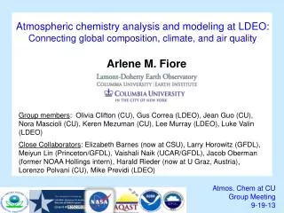
Atmospheric chemistry analysis and modeling at LDEO: Connecting global composition, climate, and air quality. Arlene M. Fiore. Group members : Olivia Clifton (CU), Gus Correa (LDEO), Jean Guo (CU), Nora Mascioli (CU), Keren Mezuman (CU), Lee Murray (LDEO), Luke Valin (LDEO)

E N D
Atmospheric chemistry analysis and modeling at LDEO: Connecting global composition, climate, and air quality Arlene M. Fiore Group members: Olivia Clifton (CU), Gus Correa (LDEO), Jean Guo (CU), Nora Mascioli (CU), KerenMezuman (CU), Lee Murray (LDEO), Luke Valin(LDEO) Close Collaborators: Elizabeth Barnes (now at CSU), Larry Horowitz (GFDL), MeiyunLin (Princeton/GFDL), VaishaliNaik (UCAR/GFDL), Jacob Oberman (former NOAA Hollings intern), HaraldRieder(now at U Graz, Austria), Lorenzo Polvani (CU), Mike Previdi (LDEO) Atmos. Chem at CU Group Meeting 9-19-13 83520601
How and why might extreme air pollution events change? pollutant sources T Fires • Need to understand how different • processes influence the distribution Mean shifts • Meteorology (e.g., stagnation vs. ventilation) Degree of mixing Variability increases • Feedbacks (Emis, Chem, Dep) OH NOx VOCs Symmetry changes PAN Deposition H2O • Changing global emissions (baseline) • Changing regional emissions (episodes) Shift in mean? Figure SPM.3, IPCC SREX 2012 Change in symmetry? Today’s Focus http://ipcc-wg2.gov/SREX/
Extreme Value Theory (EVT) methods describe the high tail of the observed ozone distribution (not true for Gaussian) JJA MDA8 O3 1987-2009 at CASTNet Penn State site EVT Approach: (Peak-over-threshold) for MDA8 O3>75 ppb Gaussian: Poor fit for extremes Observed MDA8 O3 (ppb) Observed MDA8 O3 (ppb) 1988-1998 1999-2009 Gaussian (ppb) Generalized Pareto Distribution Model (ppb) Rieder et al., ERL 2013
EVT methods enable derivation of “return levels” for JJA MDA8 O3within a given time period Return level: describes probability of observing value x (level) within time window T (period) CASTNet site: Penn State, PA 1988-1998 1999-2009 • Sharp decline in return levels • between early and later periods • (NOx SIP call) • Consistent with prior work [e.g., Frost et al., 2006; Bloomer et al., 2009, 2010] • Translates air pollution changes into • probabilistic language Rieder et al., ERL 2013 Applied methods to all EUS CASTNet sites; projections for future changes with GFDL CM3 chemistry-climate model
The GFDL CM3/AM3 chemistry-climate model Donner et al., J. Climate, 2011; Golaz et al., J. Climate, 2011 Modular Ocean Model version 4 (MOM4) & Sea Ice Model SSTs/SIC from observations or CM3 CMIP5 Simulations GFDL-AM3 GFDL-CM3 Forcing Solar Radiation Well-mixed Greenhouse Gas Concentrations Volcanic Emissions cubed sphere grid ~2°x2°; 48 levels Atmospheric Dynamics & Physics Radiation, Convection (includes wet deposition of tropospheric species), Clouds, Vertical diffusion, and Gravity wave Atmospheric Chemistry 86 km 0 km Ozone–Depleting Substances (ODS) Chemistry of Ox, HOy, NOy, Cly, Bry, and Polar Clouds in the Stratosphere 6000+ years of CM3 CMIP5 simulations [John et al., ACP, 2012 Turner et al., ACP, 2012 Levy et al., JGR, 2013 Barnes & Fiore, GRL, 2013] Options to nudge AM3 to reanalysis; also global high-res (~0.5°x0.5°) [Lin et al., JGR, 2012ab] Chemistry of gaseous species (O3, CO, NOx, hydrocarbons) and aerosols (sulfate, carbonaceous, mineral dust, sea salt, secondary organic) Pollutant Emissions (anthropogenic, ships, biomass burning, natural, & aircraft) Aerosol-Cloud Interactions Dry Deposition Naik et al., JGR, 2013 Land Model version 3 (soil physics, canopy physics, vegetation dynamics, disturbance and land use)
Generating policy-relevant statistics from biased models Average (1988-2005) number of summer days with O3 > 75 ppb Corrected CM3 simulation (regional remapping) CM3 Historical simulation (3 ensemble-member mean) CASTNet sites (observations) • Applying correction to projected simulations assumes model • captures adequately response to emission and climate changes Rieder et al., in prep
GFDL CM3 generally captures NE US JJA surface O3 decrease following NOx emission controls (-25% early 1990s to mid-2000s) Observed (CASTNet) Model (CM3) JJA MDA8 O3 (ppb) • Implies bias correction based on present-day observations can be applied to future scenarios with NOx changes (RCPs) • Caveat: Model response on low-O3 days smaller than observed Rieder et al., in prep
Climate and Emission Scenarios for the 21st Century:Representative Concentration Pathways (RCPs) Enables us to isolate role of changing climate Percentage changes from 2005 to 2100 RCP8.5 RCP4.5 RCP4.5_WMGG NE USA NOx Global NOx Global CO2 Global CH4 How will surface O3 distributions over the NE USevolve with future changes in emissions and climate? Change in Global T (°C) 2006–2025 to 2081–2100 (>500 hPa) in GFDL CM3 chemistry-climate model [John et al., ACP, 2012]
How does climate warming change extreme O3 events over the NE USA? 1-year MDA8 O3 Return Levels in GFDL CM3 RCP4.5_WMGG(corrected) Change: (2091-2100) – (2006-2015) Base Years (2006-2015) Change: (2091-2100) – (2046-2055) • Much of region sees ‘penalty’ (Wu et al., 2008) but some ‘benefit’, up to 4 ppb • Signal from regional ‘climate noise’ with only 3 ensemble members? • Robust across models? Rieder et al., in prep
Large NOx reductions offset climate penalty on O3 extremes 1-year Return Levels in CM3 chemistry-climate model (corrected) Summer (JJA) MDA8 Surface O3 [Rieder et al., in prep] 2091-2100 2046-2055 RCP4.5_WMGG: Pollutant emissions held constant (2005) + climate warming RCP4.5: Large NOxdecreases + climate warming ppb All at or below 60 ppb Nearly all at or below 70 ppb • Ongoing work examining relationship between NOx reductions and 1-year return levels Rieder et al., in prep
Does aerosol forcing influence extreme weather events? 1860-2005 “Aerosol only” forcing scenario in GFDL CM3 chemistry-climate model Warm Spell Duration (consecutive warm days) over Eastern North America Consecutive warm days Decrease in warm spell duration over ENA following increase in anthropogenic aerosol (preindustrial conditions except for aerosol) (1980-2006) – (1860-1890) N. Mascioli
Identifying key factors contributing to OH variability Can this explain large inter-model differences in OH changes (e.g., Naik et al., 2013; Voulgarakis et al. 2013)? Murray et al., 2013
Linearity with photochemical steady-state relationship holds for some models but not others: what factors are missing? Transient (CMIP5) and Time-slice (ACCMIP) simulations 1850-2100 Annual mean tropospheric [OH] (106molec cm-3) GFDL CM3 model Incorporating additional term for sulfate achieves linearity: aerosol influence on HOx sink OR correlated causal mechanism?
Space-based CH2O: often used to constrain biogenic emissions; what can we learn from background variability? Atmospheric Column CH2O as retrieved by OMI on Aura satellite Jun-Aug Dec-Feb Constraints on variability in background (CH4) oxidation? L. Valin, NOAA/LDEO
Over the Sahara, model formaldehyde columns correlate strongly with year-to-year variations in CH4 loss rates GFDL AM3 model nudged to NCEP meteorology (1981-2007) Regional averages over 20-28N, 2.5-25E Dec-Feb Exploring whether this is detectable with current space-based measurements L. Valin, NOAA/LDEO
Pollution monitoring Exposure assessment AQ forecasting Source attribution Quantifying emissions Natural & foreign influences AQ processes Climate-AQ interactions satellites AQAST suborbital platforms models AQAST
What makes AQAST unique?How is our group contributing? • All AQAST projects connect Earth Science and air quality management: • active partnerships with air quality managers with deliverables/outcomes • self-organizing to respond quickly to demands • flexibility in how it allocates its resources • INVESTIGATOR PROJECTS (IPs): members adjust work plans each year to meet evolving AQ needs • “TIGER TEAM” PROJECTS (TTs): multi-member efforts to address emerging, pressing problems requiring coordinated activity www.aqast.org: click on “projects” for brief descriptions + link to pdf describing each project • Our projects for 2013 • Stratospheric and Asian influence on inter-annual WUS surface O3 variations (M. Lin) • climate versus emissions impacts on 21stC U.S. baseline O3(seasonality) • Analysis of background O3 influence on O3 measured at new NV sites (M. Lin). • TTs (pending selection) • (PIs: Fiore, Holloway) Source attribution for high-O3 events over EUS • (PI: Streets) Satellite-derived NOx emissions and trends • In progress: Multi-model W126 analysis (vegetation exposure) • In progress: Estimates of background O3 from 2 models
Surface O3 seasonal cycle over NE USA reverses – cold season increases- under extreme warming scenario (RCP8.5) Monthly mean surface O3 (land only) over the NE USA (36-46N, 70-80W) in the GFDL CM3 model ? ppb NOx decreases 3 ensemble members for each scenario month O. Clifton
Why does surface O3 increase in winter/spring over NE USA under RCP8.5? Change in monthly mean surface O3 (land only) over the NE USA (36-46N, 70-80W) (2091-2100) – (2006-2015) RCP8.5 (3 ensemble members) ? NOx decreases ppb O. Clifton
Doubling methane raises surface O3 over NE USA ~5-10 ppb Change in monthly mean surface O3 (land only) over the NE USA (36-46N, 70-80W) (2091-2100) – (2006-2015) RCP8.5 (3 ensemble members) RCP8.5 but chemistry sees 2005 CH4 Doubling CH4 does not fully explain wintertime increase ppb O. Clifton Will the NE USA resemble present-day remote, high-altitude W US sites by 2100?
Setting achievable standards requires accurate knowledge of background levels typical U.S. “background” (model estimates) [Fiore et al., 2003; Wang et al., 2009; Zhang et al., 2011] U.S. National Ambient Air Quality Standard for O3 has evolved over time background events over WUS [Lin et al., 2012ab] 75 ppb 2008 8-hr 84 ppb 1997 8-hr 120 ppb 1979 1-hr avg Future? (proposed) O3 (ppbv) 20 60 80 40 100 120 Allowable O3 produced from U.S. anthrop. sources (“cushion”) Lowering thresholds for U.S. O3 NAAQS implies thinning cushion between regionally produced O3 and background 2008 O3 NAAQS revision relied on background estimates from one model Compare N. Amer Background in GFDL AM3 vs. GEOS-Chem
Estimates of North American background in 2 models (simulations with N. American anth. emissions set to zero) Fourth-highest North American background MDA8 O3 in model surface layer between Mar 1 and Aug 31, 2006 AM3 (~2°x2°) GEOS-Chem (½°x⅔°) J. Oberman ppb 35 42 50 57 65 Excessive lightning NOx in summer High AM3 bias in EUS; caution on N. Amer. Background here! Higher background (spring): More exchange with surface? Larger stratospheric influence? • Models robustly agree N. American background is higher at altitude in WUS • Multi-model enables error estimates, in context of observational constraints • Need to account for biases to estimate useful policy-relevant statistics Fiore et al., in prep
Connecting atmospheric composition, climate, and air quality: from background oxidation to extreme pollution events • Variability in background CH4 oxidation (OH) • Space-based constraints from formaldehyde columns? • Determine key driving factors (multi-model CMIP5/ACCMIP) Sahara region • “Climate penalty” can be offset by NOx reductions which preferentially decrease the highest O3 events • Background ozone and its specific sources over the U.S. Change in monthly mean NE USA O3 : (2091-2100) – (2006-2015) • Future shifts in regional vs. transported ozone (incl. CH4)? • Harnessing power of multiple models + observations • Variability on scales from daily to multi-decadal • Process-oriented analysis (Asian polln, strat, storms, jets) Extend to other regions, seasons, with a focus on extremes Develop robust relationships with changes in meteorology + feedbacks from the biosphere Change in 1-yr O3 RL: (2091-2100) – (2046-2055) Change in WSDI (days) (1980-2006) – (1860-1890) • New Directions • Role of aerosol forcing on extreme weather events • Process studies (lightning NOx, deposition) • Climate variability and composition