Latent Causal Modeling of Neuroimaging Data: SLCM vs. DTF Approaches
10 likes | 126 Vues
This study explores the advantages of Sparse Latent Causal Modeling (SLCM) over the Directed Transfer Function (DTF) for causal inference in neuroimaging data. SLCM potentially offers dimensionality reduction, direct constraint application on causal relations, and better handling of instantaneous mixing. We analyze a synthetic 64-channel EEG dataset, demonstrating the efficacy of SLCM in capturing latent sources and their influences on measurement channels. The findings underscore SLCM's robustness in modeling neural dynamics through Bayesian inference with sparsity priors.

Latent Causal Modeling of Neuroimaging Data: SLCM vs. DTF Approaches
E N D
Presentation Transcript
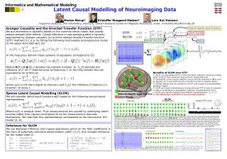
Informatics and Mathematical Modeling Latent Causal Modelling of Neuroimaging Data Lars Kai Hansen1 Morten Mørup1 Kristoffer Hougaard Madsen2 1Cognitive Systems, DTU Informatics, Denmark, 2Danish Research Centre for Magnetic Resonance, email: {mm,khm,lkh}@imm.dtu.dk Granger Causality and the Directed Transfer Function (DTF) We are interested in causality based on the common sense notion that causes always precede their effects. Causal inference in neuroimaging data is typically approached by Granger causality [4] and the related directed transfer function (DTF) method [5]., e.g. by fitting the following multivariate autoregressive model to the space-time data x(t) [5] In the frequency domain these systems of equations correspond to [5] Where H(f)=(I-Q(f))-1 denotes the transfer function. Ie. hi,j(f) denotes the influence of jth on ith channel/voxel at frequency f. In the time domain this can equivalently be written as where ej(t) is the input signal to channel j and hi,j(t) the influence of channel j to channel i at delay t. Channel Specific Input Functions Latent Sources Transfer Functions Noise e4 • Benefits of SLCM over DTF: • SLCM can potentially perform dimensionality reduction resulting in fewer latent sources than observed measurement voxels/channels. • Constraints on the causal relations can be directly imposed on A(t) such as sparsity [2,7] and restricting the transfer function to specific delays. • Spatial regions that are caused by the dth source sd(t) are automatically grouped in ad(t). • SLCM can handle instantaneous mixing whereas DTF is hard to interpret in case of instantaneous propagation between voxels/channels [4,5]. • SLCM can naturally handle overcomplete representations, i.e. I>>T. • The estimation of SLCM is a non-convex problem x4 e5 x5 e2 e3 x2 s2 x3 x6 e1 e6 s1 x1 Measurement Channel Sparse Latent Causal Modelling (SLCM) We will consider latent input functions s(t) based on the following convolutional representation Where ei(t) is residual noise. Thus measurements are caused by underlying latent sources rather than causes constrained to be the measurement channels themselves. We note that this representation corresponds to the convolutive ICA model [3, 8]. Channel Specific Input Function Latent Source SLCM Synthetic 64 channel EEG dataset. Left panel: The simulated A(t) contains two latent sources (component 1 and 2) and two components granger causing other channels (component 3 and 4). Middle panel: Estimated A(t) from a SLCM analysis. Right panel: The corresponding Granger analysis based on the DTF approach [5]. From the power of the estimated input functions e(t) of each channel it can be seen that 9 of the 64 input functions are active. The most active input functions are the input functions of channel 11 and 1 corresponding to the two channels of component 3 and 4 that were generated to Granger cause the remaining channels. Below are given the significant maximal autocorrelations (on an a=1% level) between the input functions e(t) and true simulated latent sources s(t). The estimated inputs functions to channel 11 and 1 are (correctly) significantly correlated to the latent source 3 and 4 respectively. As the DTF analysis is unable to correctly account for the dynamics of component 1 and 2 due to the instantaneous propagation between channels the information of these underlying two latent sources are arbitrarily distributed to several of the channels that observe these sources. Inference for SLCM We use Bayesian inference and impose sparseness priors on the filter coefficients in the form of automatic relevance determination (ARD) [1,7], this includes inference for the model order D. Real 64 channel EEG dataset based on visual paradigm. From the SLCM analysis a four component model was extracted. The space-time dynamics of the most prominent first component pertain to visual activation and indicate a flow from left to right occipital areas and later to more central regions.