Dynamic Causal Modelling (DCM) in Functional Neuroimaging
190 likes | 223 Vues
Explore DCM theory, parameter estimation, Bayesian methods, connectivity models, and more in functional neuroimaging analyses.

Dynamic Causal Modelling (DCM) in Functional Neuroimaging
E N D
Presentation Transcript
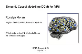
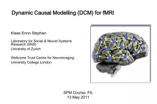
Dynamic Causal Modelling (DCM): Theory Burkhard Pleger Thanks to Klaas Enno Stephan Functional Imaging Lab Wellcome Dept. of Imaging Neuroscience Institute of Neurology University College London
Overview • DCMs as generic models of dynamic systems • Neural and hemodynamic levels in DCM • Parameter estimation • Priors in DCM • Bayesian parameter estimation • Interpretation of parameters • Bayesian model selection
System analyses in functional neuroimaging Functional specialisation Analyses of regionally specific effects: which areas constitute a neuronal system? Functional integration Analyses of inter-regional effects: what are the interactions between the elements of a given neuronal system? Functional connectivity = the temporal correlation between spatially remote neurophysiological events Effective connectivity = the influence that the elements of a neuronal system exert over another MECHANISM-FREE MECHANISTIC MODEL
Models of effective connectivity • Structural Equation Modelling (SEM) • Psycho-physiological interactions (PPI) • Multivariate autoregressive models (MAR)& Granger causality techniques • Kalman filtering • Volterra series • Dynamic Causal Modelling (DCM) Friston et al., NeuroImage 2003
Models of effective connectivity = system models.But what precisely is a system? • System = set of elements which interact in a spatially and temporally specific fashion. • System dynamics = change of state vector in time • Causal effects in the system: • interactions between elements • external inputs u • System parameters :specify the nature of the interactions • general state equation for non-autonomous systems overall system staterepresented by state variables change ofstate vectorin time
LG left FG right LG right FG left Example: linear dynamic system LG = lingual gyrus FG = fusiform gyrus Visual input in the - left (LVF) - right (RVF)visual field. z4 z3 z1 z2 RVF LVF u2 u1 systemstate input parameters state changes effective connectivity externalinputs
LG left FG right LG right FG left Extension: bilinear dynamic system z4 z3 z1 z2 CONTEXT RVF LVF u2 u3 u1
Bilinear state equation in DCM modulation of connectivity systemstate direct inputs state changes intrinsic connectivity m externalinputs
Overview • DCMs as generic models of dynamic systems • Neural and hemodynamic levels in DCM • Parameter estimation • Priors in DCM • Bayesian parameter estimation • Interpretation of parameters • Bayesian model selection
z λ y DCM for fMRI: the basic idea • Using a bilinear state equation, a cognitive system is modelled at its underlying neuronal level (which is not directly accessible for fMRI). • The modelled neuronal dynamics (z) is transformed into area-specific BOLD signals (y) by a hemodynamic forward model (λ). The aim of DCM is to estimate parameters at the neuronal level such that the modelled BOLD signals are maximally similar to the experimentally measured BOLD signals.
z λ y Conceptual overview Neural state equation The bilinear model effective connectivity modulation of connectivity Input u(t) direct inputs c1 b23 integration neuronal states a12 activity z2(t) activity z3(t) activity z1(t) hemodynamic model y y y BOLD Friston et al. 2003,NeuroImage
The hemodynamic “Balloon” model • 5 hemodynamic parameters: • Empirically determineda priori distributions. • Computed separately for each area (like the neural parameters).
LG left LG right FG right FG left Example: modelled BOLD signal Underlying model(modulatory inputs not shown) left LG right LG RVF LVF LG = lingual gyrus Visual input in the FG = fusiform gyrus - left (LVF) - right (RVF) visual field. blue: observed BOLD signal red: modelled BOLD signal (DCM)
Overview • DCMs as generic models of dynamic systems • Neural and hemodynamic levels in DCM • Parameter estimation • Priors in DCM • Bayesian parameter estimation • Interpretation of parameters • Bayesian model selection
ηθ|y stimulus function u Overview:parameter estimation neural state equation • Combining the neural and hemodynamic states gives the complete forward model. • An observation model includes measurement errore and confounds X (e.g. drift). • Bayesian parameter estimation • Result:Gaussian a posteriori parameter distributions, characterised by mean ηθ|y and covariance Cθ|y. parameters hidden states state equation observation model modelled BOLD response
needed for Bayesian estimation, embody constraints on parameter estimation express our prior knowledge or “belief” about parameters of the model hemodynamic parameters:empirical priors temporal scaling:principled prior, self-inhibition coupling parameters:shrinkage priors Priors in DCM Bayes Theorem posterior likelihood ∙ prior
Priors in DCM, self-inhibition • self-inhibition:ensured by priors on the decay rate constant σ (ησ=1, Cσ=0.105)→ these allow for neural transients with a half life in the range of 300 ms to 2 secondsNB: a single rate constant for all regions! • Identical temporal scaling in all areas by factorising A and B with σ: all connection strengths are relative to the self-connections.
system stability:in the absence of input, the neuronal states must return to a stable mode → constraints on prior variance of intrinsic connections (A) Priors in DCM, coupling • shrinkage priorsfor coupling parameters (η=0)→ conservative estimates!
Shrinkage Priors Small & variable effect Large & variable effect Small but clear effect Large & clear effect