Chapter 5 Probability Distributions

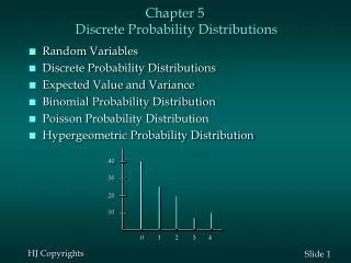
1. Chapter 5Probability Distributions 5-1 Overview 5-2 Random Variables 5-3 Binomial Probability Distributions 5-4 Mean, Variance and Standard Deviation for the Binomial Distribution 5-5 The Poisson Distribution

2. Section 5-1 Overview Created by Tom Wegleitner, Centreville, Virginia

3. This chapter will deal with the construction of discrete probability distributions by combining the methods of descriptive statistics presented in Chapter 2 and 3 and those of probability presented in Chapter 4. Probability Distributions will describe what will probably happen instead of what actually did happen. Overview

4. Combining Descriptive Methods and Probabilities In this chapter we will construct probability distributions by presenting possible outcomes along with the relative frequencies we expect.

5. Section 5-2 Random Variables Created by Tom Wegleitner, Centreville, Virginia

6. Key Concept This section introduces the important concept of a probability distribution, which gives the probability for each value of a variable that is determined by chance. Give consideration to distinguishing between outcomes that are likely to occur by chance and outcomes that are “unusual” in the sense they are not likely to occur by chance.

7. Random variable a variable (typically represented by x) that has a single numerical value, determined by chance, for each outcome of a procedure Probability distribution a description that gives the probability for each value of the random variable; often expressed in the format of a graph, table, or formula Definitions

8. Discrete random variable either a finite number of values or countable number of values, where “countable” refers to the fact that there might be infinitely many values, but they result from a counting process Definitions • Continuous random variable infinitely many values, and those values can be associated with measurements on a continuous scale in such a way that there are no gaps or interruptions

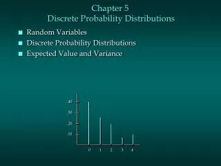
9. Graphs The probability histogram is very similar to a relative frequency histogram, but the vertical scale shows probabilities.

10.  P(x) = 1 where x assumes all possible values. Requirements for Probability Distribution • 0 P(x) 1 • for every individual value of x.

11. µ=[x•P(x)] Mean 2=[(x –µ)2 • P(x)] Variance 2=[x2 • P(x)] –µ2Variance (shortcut) = [x2 • P(x)] –µ2Standard Deviation Mean, Variance and Standard Deviation of a Probability Distribution

12. Round results by carrying one more decimal place than the number of decimal places used for the random variable x. If the values of xare integers, round µ, ,and2 to one decimal place. Roundoff Rule for µ,,and2

13. Identifying Unusual Results Range Rule of Thumb According to the range rule of thumb, most values should lie within 2 standard deviations of the mean. We can therefore identify “unusual” values by determining if they lie outside these limits: Maximum usual value = μ + 2σ Minimum usual value = μ – 2σ

14. Identifying Unusual Results Probabilities Rare Event Rule If, under a given assumption (such as the assumption that a coin is fair), the probability of a particular observed event (such as 992 heads in 1000 tosses of a coin) is extremely small, we conclude that the assumption is probably not correct. • Unusually high: x successes among n trials is an unusually high number of successes if P(x or more) ≤ 0.05. • Unusually low: x successes among n trials is an unusually low number of successes if P(x or fewer) ≤ 0.05.

15. Definition The expected value of a discrete random variable is denoted by E, and it represents the average value of the outcomes. It is obtained by finding the value of  [x• P(x)]. E =  [x• P(x)]

16. Recap In this section we have discussed: • Combining methods of descriptive statistics with probability. • Random variables and probability distributions. • Probability histograms. • Requirements for a probability distribution. • Mean, variance and standard deviation of a probability distribution. • Identifying unusual results. • Expected value.

17. Section 5-3 Binomial Probability Distributions Created by Tom Wegleitner, Centreville, Virginia

18. Key Concept This section presents a basic definition of a binomial distribution along with notation, and it presents methods for finding probability values. Binomial probability distributions allow us to deal with circumstances in which the outcomes belong to two relevant categories such as acceptable/defective or survived/died.

19. Definitions A binomial probability distribution results from a procedure that meets all the following requirements: 1. The procedure has a fixed number of trials. 2. The trials must be independent. (The outcome of any individual trial doesn’t affect the probabilities in the other trials.) 3. Each trial must have all outcomes classified into twocategories (commonly referred to as success and failure). 4. The probability of a success remains the same in all trials.

20. Notation for Binomial Probability Distributions S and F (success and failure) denote two possible categories of all outcomes; p and q will denote the probabilities of S and F, respectively, so P(S) = p (p = probability of success) P(F) = 1 – p = q (q = probability of failure)

21. Notation (cont) n denotes the number of fixed trials. x denotes a specific number of successes in n trials, so x can be any whole number between 0 and n, inclusive. p denotes the probability of success in one of the n trials. q denotes the probability of failure in one of the n trials. P(x) denotes the probability of getting exactly x successes among the n trials.

22. When sampling without replacement, consider events to be independent if n < 0.05N. Important Hints • Be sure that x and p both refer to the same category being called a success.

23. Methods for Finding Probabilities We will now discuss three methods for finding the probabilities corresponding to the random variable x in a binomial distribution.

24. n! P(x) = •px•qn-x (n –x)!x! for x = 0, 1, 2, . . ., n Method 1: Using the Binomial Probability Formula where n = number of trials x = number of successes among n trials p = probability of success in any one trial q = probability of failure in any one trial (q = 1 – p)

25. Method 2: Using Table A-1 in Appendix A Part of Table A-1 is shown below. With n = 12 and p = 0.80 in the binomial distribution, the probabilities of 4, 5, 6, and 7 successes are 0.001, 0.003, 0.016, and 0.053 respectively.

26. Method 3: Using Technology STATDISK, Minitab, Excel and the TI-83 Plus calculator can all be used to find binomial probabilities. STATDISK Minitab

27. Method 3: Using Technology STATDISK, Minitab, Excel and the TI-83 Plus calculator can all be used to find binomial probabilities. Excel TI-83 Plus calculator

28. Strategy for Finding Binomial Probabilities • Use computer software or a TI-83 Plus calculator if available. • If neither software nor the TI-83 Plus calculator is available, use Table A-1, if possible. • If neither software nor the TI-83 Plus calculator is available and the probabilities can’t be found using Table A-1, use the binomial probability formula.

29. n! P(x) = •px•qn-x (n –x )!x! The number of outcomes with exactly x successes among n trials Rationale for the Binomial Probability Formula

30. n! P(x) = •px•qn-x (n –x )!x! The probability of x successes among n trials for any one particular order Number of outcomes with exactly x successes among n trials Binomial Probability Formula

31. Recap In this section we have discussed: • The definition of the binomial probability distribution. • Notation. • Important hints. • Three computational methods. • Rationale for the formula.

32. Section 5-4 Mean, Variance, and Standard Deviation for the Binomial Distribution Created by Tom Wegleitner, Centreville, Virginia

33. Key Concept In this section we consider important characteristics of a binomial distribution including center, variation and distribution. That is, we will present methods for finding its mean, variance and standard deviation. As before, the objective is not to simply find those values, but to interpret them and understand them.

34. Meanµ = [x•P(x)] Variance2= [x2•P(x) ] –µ2 Std. Dev = [x2•P(x) ] –µ2 For Any Discrete Probability Distribution: Formulas

35. Meanµ = n•p Variance2 = n•p•q Std. Dev. = n • p • q Binomial Distribution: Formulas Where n = number of fixed trials p = probability of success in one of the n trials q = probability of failure in one of the n trials

36. Maximum usual values = µ + 2 Minimum usual values = µ– 2  Interpretation of Results It is especially important to interpret results. The range rule of thumb suggests that values are unusual if they lie outside of these limits:

37. Recap In this section we have discussed: • Mean,variance and standard deviation formulas for the any discrete probability distribution. • Mean,variance and standard deviation formulas for the binomial probability distribution. • Interpreting results.

38. Section 5-5 The Poisson Distribution Created by Tom Wegleitner, Centreville, Virginia

39. Key Concept The Poisson distribution is important because it is often used for describing the behavior of rare events (with small probabilities).

40. The Poisson distribution is a discrete probability distribution that applies to occurrences of some event over a specified interval. The random variablex is the number of occurrences of the event in an interval. The interval can be time, distance, area, volume, or some similar unit. Formula µx• e -µ P(x) = wheree  2.71828 x! Definition

41. The random variable x is the number of occurrences of an event over some interval. The occurrences must be random. The occurrences must be independent of each other. The occurrences must be uniformly distributed over the interval being used. Parameters The mean is µ. • The standard deviation is  = µ . Poisson Distribution Requirements

42. Difference from a Binomial Distribution The Poisson distribution differs from the binomial distribution in these fundamental ways: • The binomial distribution is affected by the sample size n and the probability p, whereas the Poisson distribution is affected only by the mean μ. • In a binomial distribution the possible values of the random variable x are 0, 1, . . . n, but a Poisson distribution has possible x values of 0, 1, . . . , with no upper limit.

43. Rule of Thumb n 100 np 10 Poisson as Approximation to Binomial The Poisson distribution is sometimes used to approximate the binomial distribution when n is large and p is small.

44. n 100 np 10 Poisson as Approximation to Binomial - μ Value for μ = n • p

45. Recap In this section we have discussed: • Definition of the Poisson distribution. • Requirements for the Poisson distribution. • Difference between a Poisson distribution and a binomial distribution. • Poisson approximation to the binomial.