Understanding the Hilbert Transform in EOF Analysis of Linear Systems
150 likes | 271 Vues
This document explores the application of the Hilbert Transform to analyze Eigenfunction Orthogonal Functions (EOFs) in linear systems. It details how the Hilbert Transform produces a complex variable with a real part identical to the original time series and an imaginary part that is phase-shifted by 90 degrees. We provide a practical example using MATLAB to visualize a sinusoidal signal and its associated Hilbert Transform. The process enhances the understanding of signal phase propagation and the characteristics of the EOF analysis.

Understanding the Hilbert Transform in EOF Analysis of Linear Systems
E N D
Presentation Transcript
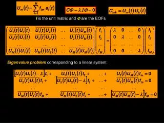
I is the unit matrix and are the EOFs Eigenvalue problemcorresponding to a linear system:
Sometimes use another complex form of EOFS. Apply the Hilbert Transformof U to understand a bit more about the phase of propagation of the phenomenon In essence, the Hilbert transform of a signal (time series) produces a complex variable with real part identical to the time series and the imaginary part is shifted 90º from the original (sometimes called the analytical signal): >> t=[1:1:1000]; >> u1=sin(2*pi*t/200); >> plot(t,u1,’LineWidth’,3) u1 t
>> t=[1:1:1000]; >> u1=sin(2*pi*t/200); >> plot(t,u1,’LineWidth’,3) >> >> u2=hilbert(u1); >> hold on; >> plot(real(u2),'r--','LineWidth',3) u t
>> t=[1:1:1000]; >> u1=sin(2*pi*t/200); >> plot(t,u1,’LineWidth’,3) >> >> u2=hilbert(u1); >> hold on >> plot(real(u2),'r--','LineWidth',3) >> plot(imag(u2),'g','LineWidth',3) u t
Hilbert Transformof U can be regarded as the convolution of U with h(t) = 1/(t) P is the Cauchy principal value (assigns values to improper integrals) • hilbert uses a four-step algorithm: • 1. It calculates the FFT of the input sequence, storing the result in a vector x. • 2. It creates a vector h whose elements h(i) have the values: • 1 for i = 1, (n/2)+1 • 2 for i = 2, 3, ... , (n/2) • 0 for i= (n/2)+2, ... , n • 3. It calculates the element-wise product of x and h. • 4. It calculates the inverse FFT of the sequence obtained in step 3 and returns the first n elements of the result.
Mean Profile 10 log (echo)
18% 60% 9%
Hilbert EOF 18% 6% 64%