Comprehensive Guide to Matrix Manipulation and 2D Plotting in MATLAB
This guide covers essential concepts in matrix manipulation and 2D plotting using MATLAB. It starts with basic matrix entry, generation of arrays, and manipulating matrix entries. We explore linear systems solving, functions for data loading, and customization of plots, including titles, labels, and legends. It includes examples such as creating magic squares, plotting mathematical functions, and loading CSV data. Additionally, it discusses various plotting attributes and how to manage multiple plots within a single figure, making it a valuable resource for beginners and intermediate users alike.

Comprehensive Guide to Matrix Manipulation and 2D Plotting in MATLAB
E N D
Presentation Transcript
Review • Command Line • Semi Colon to suppress output • X = 3; • Entering a Matrix • Square brackets • X = [1,2,3,4,5] • Generate arrays (1D matrices) • X = Start:Step:End • X = 1:3:13
Matrix Manipulation • The basic unit of data storage • Extract a part of a matrix use round brackets • third entry in a 1D matrix • X(3) • last Entry • X(end) • fourth to ninth entries • X(4:9) • A 2D matrix • Entry at the third row, second column • A(3,2) • All of the third row • A(3,:)
Examples • Create a 5 by 5 magic square • There is a inbuilt function • Extract the value at the third row, fourth column • Extract the last value of the third column • Extract all of the fifth row • Replace the value at row 2, column 4 with 100 • Replace all of the first column with zeros • Delete all of the fourth row A = magic(5) A(3,4) A(end,3) A(5,:) A(2,4)=100 A(:,1)=0 A(4,:)=[]
Questions • What do the following command do? • If A is a 2D matrix • A' • B = [A';A'] • A(:)
Solving linear Systems • Represent in matrix form • Use backslash operator • Inv(A)*b • A/b
2D Plotting • Various, flexible, plotting routines. • The basic command is • plot(x,y) • This plots the vector of x coordinates against the vector of y coordinates • X and y must be the same size • plot(y) • Plots the vector y against its indices
Plotting • Plot the function y = sin(x) +x -2 • for x = [-2,9] x= -2:0.1:9; y = sin(x)+ x-2; plot(x,y)
Plot the following • y = 0.2* e-0.1x • for x = [-1,1] • y = sin(x) +x^2 -2 • for x = [-5,10]
Data Loading • Navigate to appropriate directory • Right click on file and select importdata • If in plain text format • A = Load(‘file name.???’); • If a other formats (eg. Excel files) • A = importdata(‘file name.xls’);
Data Loading Tasks • Download and then load data file • https://files.warwick.ac.uk/kimmckelvey/files/CVBulk.tsv • Load CVBulk.tsv data • Create a plot of this data
>> data = load('c:/CVBulk.tsv'); >> figure >> plot(data(:,1),data(:,2),'r') >> title('CV') >> xlabel('Voltage / V') >> ylabel('Current / A')
Changing Attributes • Basic usage: plot(x, y, ’Attributes’) • To plot a green dashed line • plot(x, y, ’g--’) • To plot yellow circle at the data points • plot(x, y, ‘yo’)
Titles etc • Adding a title • Title(‘whoop whoop’) • Axes labels • xlabel(‘Peanuts’) • ylabel(‘Vanilla’) • Legend • legend('222','33')
Multiple • To plot multiple line of the same plot • plot(X,Y,'y-',X1,Y1,'go') • Or use the ‘hold on’ function • plot(x, y, ’b.’) • hold on • plot(v, u, ‘r’)
Subplot • Used to plot multiple graphs in the same frame • Try: • Plot sine and cosine between 0 and 10 on two separate axes in the same frame >> subplot(2,1,1) >> plot(x, y) >> subplot(2,1,2) >> plot(u, v)
More attributes: • Plots are fully editable from the figure window. Once you have a plot, you can click Tools->Edit plot to edit anything. • plot(X1,Y1,LineSpec,'PropertyName',PropertyValue) • Plot(x, y, ’r’, ‘LineWidth’, 3, ‘MarkerSize',10) • But all this can also be done from the command line • set(gca,'XTick',-pi:pi/2:pi)
More types of plots • Histograms • Bar • Pie Charts • Create a bar plot of the CVBulk data
Task • Plot the following equations on the same graph (different colours) • Solve the system of equations • Plot the solution on the same graph • Add appropriate titles, labels and legend