Queueing Analysis of Production Systems (Factory Physics)
860 likes | 1.26k Vues
Queueing Analysis of Production Systems (Factory Physics). Reading Material. Chapter 8 from textbook Handout: Single Server Queueing Model by Wallace Hopp (available for download from class website). Queueing analysis is a tool for evaluating operational performance Utilization

Queueing Analysis of Production Systems (Factory Physics)
E N D
Presentation Transcript
Queueing Analysis of Production Systems (Factory Physics)
Reading Material • Chapter 8 from textbook • Handout: Single Server Queueing Model by Wallace Hopp (available for download from class website)
Queueing analysis is a tool for evaluating operational performance • Utilization • Time-in-system (flow time, leadtime) • Throughput rate (production rate, output rate) • Waiting time (queueing time) • Work-in-process (number of parts or batches in the systems)
A Single Stage System Finished parts Raw material Processing unit
The Queueing Perspective Departure (completion) of jobs Arrival (release) of jobs Queue (logical or physical) of jobs Server (production facility)
System Parameters • E[A]: average inter-arrival time between consecutive jobs • l: arrival rate (average number of jobs that arrive per unit time), l = 1/E[A] • E[S]: average processing time • m: processing rate (maximum average number of jobs that can be processed per unit time), m = 1/E[S] • r: average utilization, r = E[S]/E[A] = l/m
Performance Measures • E[W]: average time a job spends in the system • E[Wq]: average time a job spends in the queue • E[N]: average number of job in the system (average WIP in the system) • E[Nq]: average number of jobs in the queue (average WIP in the queue) • TH: throughput rate (average number of jobs produced per unit time)
Performance Measures (Continued…) E[W] = E[Wq] + E[S] E[N] = E[Nq] + r
Little’s Law E[N] = lE[W] E[Nq] = lE[Wq] r = lE[S]
Example 1 • Jobs arrive at regular & constant intervals • Processing times are constant • Arrival rate < processing rate (l < m)
Example 1 • Jobs arrive at regular & constant intervals • Processing times are constant • Arrival rate < processing rate (l < m) • E[Wq] = 0 • E[W] = E[Wq] + E[S] = E[S] • r = l/m • E[N] = lE[W] = lE[S] = r • E[Nq] = lE[Wq]= 0 • TH = l
Case 2 • Jobs arrive at regular & constant intervals • Processing times are constant • Arrival rate > processing rate (l > m)
Case 2 • Jobs arrive at regular & constant intervals • Processing times are constant • Arrival rate > processing rate (l > m) • E[Wq] = • E[W] = E[Wq] + E[S] = • r = 1 • E[N] = lE[W] = • E[Na] = lE[Wa] = • TH = m
Case 3 • Job arrivals are subject to variability • Processing times are subject to variability • Arrival rate < processing rate (l < m) • Example: Average processing time = 6 min Inter-arrival time = 8 min
Case 3 (Continued…) • r = 6/8 = 0.75 • TH = 1/8 job/min = 7.5 job/hour • E[Wq] > 0 • E[W] > E[S] • E[Nq] > 0 • E[N] > r
In the presence of variability, jobs may wait for processing and a queue in front of the processing unit may build up. • Jobs should not be released to the system at a faster rate than the system processing rate.
Sources of Variability Sources of variability include: • Demand variability • Processing time variability • Batching • Setup times • Failures and breakdowns • Material shortages • Rework
Variability Classes Low variability (LV) Moderate variability (MV) High variability (HV) CV 0 0.75 1.33
Illustrating Arrival Variability Low variability arrivals t High variability arrivals t
The G/G/1 Queue If (1) l< m, (2) the distributions of job processing and inter-arrival times are independent and identically distributed (iid), and (3) jobs are processed on a first come, first served (FCFS) basis, then average waiting time in the queue can be approximated by the “VUT” formula:
Example • CA = CS = 1 • E[S] = 1 • Case 1: r = 0.50 E[W] = 2, E[N] = 1 • Case 2: r = 0.66 E[W] = 3, E[N] = 1.98 • Case 2: r = 0.75 E[W] = 4, E[N] = 3 • Case 1: r = 0.80 E[W] = 5, E[N] = 4 • Case 1: r = 0.90 E[W] = 10, E[N] = 9 • Case 1: r = 0.95 E[W] = 20, E[N] = 19 • Case 1: r = 0.99 E[W] = 100, E[N] = 99
Example • CA = 1 • E[S] = 1 • r = 0.8 • Case 1: CS = 0 E[W]= 3, E[N] = 2.4 • Case 2: CS= 0.5 E[W] = 4, E[N] = 3.2 • Case 1: CS = 1 E[W] = 5, E[N] = 4 • Case 1: CS = 1.5 E[W] = 6, E[N] = 4.8 • Case 1: CS = 2 E[W] = 7, E[N] = 5.6
Facilities should not be operated near full capacity. • To reduce time in system and WIP, we should allow for excess capacity or reduce variability (or both).
A Single Stage System with Parallel facilities Departure (completion) of jobs Arrival (release) of jobs Queue (logical or physical) of jobs Servers (production facilities)
The G/G/m Queue If (1) l< mm, (2) the distributions of job processing and inter-arrival times are independent and identically distributed (iid), and (3) jobs are processed on a first come, first served (FCFS) basis, then average waiting time in the queue can be approximated by the “VUT” formula:
Increasing Capacity • Capacity can be increased by either increasing the production rate (decreasing processing times) or increasing the number of production facilities
Increasing Capacity • Capacity can be increased by either increasing the production rate (decreasing processing times) or increasing the number of production facilities • In a system with multiple parallel production facilities,maximum throughput equals the sum of the production rates
Dedicated versus Pooled Capacity • Dedicated system: m production facilities, each with a single processor with production rate m and arrival rate l • Pooled system: A single production facility with mparallel processors, with production rate m per processor, and arrival rate ml
Dedicated versus Pooled Capacity • Dedicated system: • Pooled system:
Pooling reduces expected waiting time by more than a factor of m • Pooling makes better use of existing capacity by continuously balancing the load among different processors
A Common Notation GX/GY/k/N N: maximum number of customers allowed G: distribution of inter-arrival times G: distribution of service times k: number of servers X: distribution of arrival batch (group) size Y: distribution of service batch size
Common examples M/M/1 M/G/1 M/M/k M/M/1/N MX/M/1 GI/M/1 M/M/k/k
Notation in the Book versus Notation in the Lecture Notes • CT (cycle time): E(W) • CTq (cycle time in the queue): E(Wq) • WIP: E(N) • WIPq (WIP in the queue): E(Nq) • u: U (r =l/m) • ra: l • te: E(S); ts: E(X); • ca: cA • ce: cS
Assumptions • A single server queue • The distribution of inter-arrival times is exponential (Markovian arrivals) • The distribution of processing times is exponential (Markovian processing times)
Exponential Inter-arrival Times and the Poisson Process Poisson distribution
The Birth-Death Model l l l 0 1 2 3 m m m