Download

1 / 23
240 likes | 494 Vues
The PRECIS Regional Climate Model. General overview (1). The regional climate model (RCM) within PRECIS is a model of the atmosphere and land surface, of limited area and high resolution and locatable over any part of the globe. The Hadley Centre’s most up to date model: HadRM3P.

E N D
General overview (1) • The regional climate model (RCM) within PRECIS is a model of the atmosphere and land surface, of limited area and high resolution and locatable over any part of the globe. • The Hadley Centre’s most up to date model: HadRM3P
General overview (2) • The advective and thermodynamical evolution of atmospheric pressure, winds, temperature and moisture (prognostic variables) are simulated, whilst including the effects of many other physical processes. • Other useful meteorological quantities (diagnostic variables) are derived consistently within the model from the prognostic variables • precipitation, cloud coverage, …
° time Discretizing the model equations • All model equations are solved numerically on a discrete 3-dimensional grid spanning the area of the model domain and the depth of the atmosphere • The model simulates values at discrete, evenly spaced points in time • The period between each point in time is called the model’s timestep • Spatially, data is an average over a grid box • Temporally, data is instantaneous
The model grid • Hybrid vertical coordinate • Combination of terrain following and atmospherics pressure • 19 vertical levels (lowest at 50m, highest at 5Pa) • Regular lat-lon grid in the horizontal • ‘Arakawa B’ grid layout • P = pressure, temperature and moisture related variables • W = wind related variables
Physical parameterizations • Clouds and precipitation • Radiation • Atmospheric aerosols • Boundary layer • Land surface • Gravity wave drag
Large scale clouds and precipitation • Resulting from the large scale movement of air masses affecting grid box mean moisture levels • Due to dynamical assent (and radiative cooling and turbulent mixing) • Cloud water and cloud ice are simulated • Conversion of cloud water to precipitation depends on • the amount of cloud water present • precipitation falling into the grid box from above (seeder-feeder enhancement) • Precipitation can evaporate and melt
Convection and convective precipitation • Cloud formation is calculated from the simulated profiles of • temperature • pressure • humidity • aerosol particle concentration • Entrainment and detrainment • Anvils of convective plumes are represented
Radiation • The daily, seasonal and annual cycles of incoming heat from the sun (shortwave insolation) are simulated • Short-wave and long-wave energy fluxes modelled separately • SW fluxes depend on • the solar zenith angle, absorptivity (the fraction of the incident radiation absorbed or absorbable), albedo(reflected radiation/incident radiation) and scattering(deflection) ability • LW fluxes depend on • the amountan emitting medium that is present, temperatureandemissivity (radiation emitted/radiation emitted by a black body of the same temperature) • Radiative fluxes are modelled in 10 discrete wave bands spanning the SW and LW spectra • 4 SW, 6 LW
Atmospheric aerosols • The spatial distribution and life cycle of atmospheric sulphate aerosol particles are simulated • Other aerosols (e.g. soot, mineral dust) are not included • Sulphate aerosol particles (SO4) tend to give a surface cooling: • The direct effect (scattering of incoming solar radiation more solar radiation reflected back to space) • The first indirect effect (increased cloud albedo due to smaller cloud droplets more solar radiation reflected back to space) • Natural and anthropogenic emissions are prescribed source terms (scenario specific)
Boundary layer processes • Turbulent mixing in the lower atmosphere • Sub-gridscale turbulence mixes heat, moisture and momentum through the boundary layer • The extent of this mixing depends on the large scale stability and nature of the surface • Vertical fluxes of momentum • ground atmosphere • Fluxes depend on atmospheric stability and roughness length
q, T q, T q, T q, T q, T q, T Surface processes: MOSES I • Exchange of heat and moisture between the earth’s surface, vegetation and atmosphere • Surface fluxes of heat and moisture • Precipitation stored in the vegetation canopy • Released to soil or atmosphere • Depends on vegetation type • Heat and moisture exchanges between the (soil) surface and the atmosphere pass through the canopy • Sub-surface fluxes of heat and moisture in the soil • 4 layer soil model • Root action (evapotranspiration) • Water phase changes • Permeability depending on soil type • Run-off of surface and sub-surface water to the oceans ,
Lateral Boundary Conditions (LBCs) • LBCs = Meteorological boundary conditions at the lateral (side) boundaries of the RCM domain • They constrain the prognostic variables of the RCM throughout the simulation • ‘Driving data’ comes from a GCM or analyses • Lateral Boundary condition variables: • Wind • Temperature • Water vapour • Surface pressure • Sulphur variables (if using the sulphur cycle)
Other boundary conditions • Information required by the model for the duration of a simulation • They are: • Constant data applied at the surface • Land-sea mask • Orographic fields (e.g. surface heights above sea level, 3-D s.d. of altitude) • Vegetation and soil characteristics (e.g. surface albedo, height of canopy) • Time varying data applied at the surface • SST and SICE fractions • Anthropogenic SO2 emissions (sulphur cycle only) • Dimethyl sulphide (DMS) emissions (sulphur cycle only) • Time varying data applied throughout the atmosphere • Atmospheric ozone (O3) • Constant data applied throughout the atmosphere • Natural SO2 emissionsvolcanos (sulphur cycle only) • Annual cycle data applied throughout the atmosphere • Chemical oxidants (OH, HO2, H2O2, O3) (sulphur cycle only)
Understanding Jhelum river Pakistan rainfall during the 1992 flood Observed 50km RCM 25km RCM Observed 50km RCM 25km RCM
Precipitation estimates over Eastern Africa Current climate (1961-1990) PRECIS NCEP-Reanalysis Captures the regional rainfall pattern along the East African steep topography and Red Sea area Future projections: 2080s July rainfall 2080 -B2 July rainfall 2080 -A2 • Increased rainfall (1.5mm/day) over the domain for both A2 & B2 • More areas in A2 would experience higher rainfall increases
Summer daily temperature changes: 2080 Minimum Maximum Change in mean minimum Subtropical Subtropical Tropical Tropical Change in mean maximum Equatorial Equatorial
Projected changes in future climates for 2080 under B2 scenario over China Annual mean temp. Annual mean precip. • Precipitation would increase over most areas of China (mid. of south, north and Tibetan plateau) and decrease over the northeast. • Over all temperature increase with a south-north gradient (up to 5oC). • Increasing JJA precip. Amounts within Yangtze Basin would increase frequency of flooding. • Decreasing precip. in Yellow Basin and the north,coupled with increasing temp. would enhance drought in these areas. Mean DJF precip. Mean DJF temp. Mean JJA temp. Mean JJA precip.
Change in ground-nut yields over India Ratio of simulated to observed mean (left) of yield for the baseline simulation with Topt=28oC. Percentage change in mean yield for 2071-2100 relative to baseline:TOL-28 (bottom left) & TOL-36 (bottom right). Over 70% reduction in some areas.
Climate Impacts Uncertainty Changes in 50-year flood (%) from different drivers: River Beult in Kent Natural variability – resampling: -34 to +17 Emissions – B1 to A1FI: -14 to - 9 GCM structure – 5 GCMs: -13 to +41 Natural variability – 3xGCM ICs: -25 to - 5 Downscaling – RCM v statistical: -22 to - 8 RCM structure – 8 RCMs: -5 to +8 Hydro’ model structure – 2 models: -45 to - 22 Hydro’ model parameters: +1 to + 7 % change in flood frequency Q1: Are ranges additive? Q2: Should model or observed climates be used as the baseline? Q3: Are flow changes reliable enough to apply to observed flows? Q4: Do reliable changes require full spectrum variability changes?