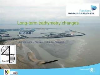
Long-term bathymetry changes
Long-term bathymetry changes. Job Janssens – Flanders Hydraulics Research. Quest4D. Outline. Available data Interpolation concerns methodology results Analysis of the grids visualization of the depth lines trend analysis chart differencing conclusions.

Long-term bathymetry changes
E N D
Presentation Transcript
Long-term bathymetry changes Job Janssens – Flanders Hydraulics Research Quest4D
Outline • Available data • Interpolation concerns methodology results • Analysis of the grids visualization of the depth lines trend analysis chart differencing conclusions
Available data Selection of historical navigation charts: (charts available at Hydrography Department, Flemish Authorities) 2007 chart high resolution grid (20m x 20m) other charts irregular pattern of data points
Available data Example:Chart of 1938
Available data Example:Chart of 1938 datapoints 1938digitized in ArcGIS
Available data Example:Chart of 1938 datapoints 1938digitized in ArcGIS datapoints 1908digitized in ArcGIS
Available data Example:Chart of 1938 different charts have datapoints on different locationsinterpolation of each set of datapoints to a grid datapoints 1938digitized in ArcGIS datapoints 1908digitized in ArcGIS
Interpolation: concerns Problems associated with interpolation: ArcGIS interpolation techniques: IDW kriging natural neighbor are averaging techniques average value cannot be greater than highest or less than lowest input in sparse data sets: interpolation cannot reproduce ridges or troughs! seafloor morphology flattened by interpolation
Interpolation: concerns “straightforward” interpolation: test case • 2007 data point set: • - high resolution (20m x 20m) • - no interpolation needed
Interpolation: concerns “straightforward” interpolation: test case • 2007 data point set: • - high resolution (20m x 20m) • - no interpolation needed • subset of the 2007 data point set
Interpolation: concerns “straightforward” interpolation: test case • 2007 data point set: • - high resolution (20m x 20m) • - no interpolation needed • subset of the 2007 data point set • interpolation of this subset
Interpolation: concerns “straightforward” interpolation: test case difference chart: 2007 - 2007 interpolated • ridges less higher than they are • troughs less deeper than they are Conclusion: interpolation of sparse data set flattens morphology interpolation error correlated with location
Interpolation: methodology Solution: use high resolution data of 2007 to estimate interpolation error Example: grid of 1938 data points of 2007, but only at locations of the 1938 data points _ _ interpolation of data points 1938 interpolation of sub- set data points 2007 = grid of 1938 grid of 2007 estimation of inter- polation error ! Basic assumption: stable morphology: no major changes in location of ridges/troughs
Analysis of the grids • visualization of different depth lines • trend analysis • chart differencing Erosion/sedimentation patterns studied through:
Analysis of the grids 1) visualization of depth lines: Example: Middelkerkebank, 8m depth lines
Analysis of the grids 2) Trend analysis: linear least square fit on time series of depth values (time series of 5 depth values for each grid cell) sedimentation trend ~ 0.03 m/year
Analysis of the grids 2) Trend analysis:
Analysis of the grids 3) Chart differencing:
Analysis of the grids Morphologic changes: Conclusions: • Anthropogenic: dredging: of navigation channels (Scheur, Pas van ‘t Zand) dumping: S1 (Sierra Ventana), … influence of breakwaters Zeebrugge harbour: bay of Heist • Natural: no significant movement of the banks sedimentation/erosion: coastal banks form the most dynamic zone sedimentation of the ridges (e.g. Oostendebank) erosion of the troughs (e.g. Grote Rede, Kleine Rede)