Download

1 / 49
490 likes | 625 Vues
Explore the essential concepts of data warehousing, a rapidly growing industry valued at $8 billion since 1998. This overview covers the purpose and models of data warehouses, including OLAP and OLTP processing. Learn about the benefits of implementing data warehouses, such as high query performance and historical data integration. Dive into architectural components, metadata, and practical applications like forecasting and performance monitoring. Discover future directions and the evolving landscape of data warehousing.

E N D
Data Warehousing CPS216Notes 13 Shivnath Babu
Warehousing • Growing industry: $8 billion way back in 1998 • Range from desktop to huge: • Walmart: 900-CPU, 2,700 disk, 23TBTeradata system • Lots of buzzwords, hype • slice & dice, rollup, MOLAP, pivot, ...
Outline • What is a data warehouse? • Why a warehouse? • Models & operations • Implementing a warehouse • Future directions
more What is a Warehouse? • Collection of diverse data • subject oriented • aimed at executive, decision maker • often a copy of operational data • with value-added data (e.g., summaries, history) • integrated • time-varying • non-volatile
What is a Warehouse? • Collection of tools • gathering data • cleansing, integrating, ... • querying, reporting, analysis • data mining • monitoring, administering warehouse
Client Client Query & Analysis Warehouse Integration Source Source Source Warehouse Architecture Metadata
Motivating Examples • Forecasting • Comparing performance of units • Monitoring, detecting fraud • Visualization
? Source Source Why a Warehouse? • Two Approaches: • Query-Driven (Lazy) • Warehouse (Eager)
Client Client Mediator Wrapper Wrapper Wrapper Source Source Source Query-Driven Approach
Advantages of Warehousing • High query performance • Queries not visible outside warehouse • Local processing at sources unaffected • Can operate when sources unavailable • Can query data not stored in a DBMS • Extra information at warehouse • Modify, summarize (store aggregates) • Add historical information
Advantages of Query-Driven • No need to copy data • less storage • no need to purchase data • More up-to-date data • Query needs can be unknown • Only query interface needed at sources • May be less draining on sources
OLTP: On Line Transaction Processing Describes processing at operational sites OLAP: On Line Analytical Processing Describes processing at warehouse OLTP vs. OLAP
Mostly updates Many small transactions Mb-Gb of data Raw data Clerical users Up-to-date data Consistency, recoverability critical Mostly reads Queries long, complex Gb-Tb of data Summarized, consolidated data Decision-makers, analysts as users OLTP vs. OLAP OLTP OLAP
Data Marts • Smaller warehouses • Spans part of organization • e.g., marketing (customers, products, sales) • Do not require enterprise-wide consensus • but long term integration problems?
Warehouse Models & Operators • Data Models • relations • stars & snowflakes • cubes • Operators • slice & dice • roll-up, drill down • pivoting • other
Terms • Fact table • Dimension tables • Measures
Dimension Hierarchies sType store city region è snowflake schema è constellations
Cube Fact table view: Multi-dimensional cube: dimensions = 2
day 2 day 1 3-D Cube Fact table view: Multi-dimensional cube: dimensions = 3
ROLAP vs. MOLAP • ROLAP:Relational On-Line Analytical Processing • MOLAP:Multi-Dimensional On-Line Analytical Processing
Aggregates • Add up amounts for day 1 • In SQL: SELECT sum(amt) FROM SALE • WHERE date = 1 81
Aggregates • Add up amounts by day • In SQL: SELECT date, sum(amt) FROM SALE • GROUP BY date
Another Example • Add up amounts by day, product • In SQL: SELECT date, sum(amt) FROM SALE • GROUP BY date, prodId rollup drill-down
Aggregates • Operators: sum, count, max, min, median, ave • “Having” clause • Using dimension hierarchy • average by region (within store) • maximum by month (within date)
rollup drill-down Cube Aggregation Example: computing sums day 2 . . . day 1 129
Cube Operators day 2 . . . day 1 sale(c1,*,*) 129 sale(c2,p2,*) sale(*,*,*)
Extended Cube * day 2 sale(*,p2,*) day 1
day 2 day 1 Aggregation Using Hierarchies customer region country (customer c1 in Region A; customers c2, c3 in Region B)
day 2 day 1 Pivoting Fact table view: Multi-dimensional cube: Pivot turns unique values from one column into unique columns in the output
Derived Data • Derived Warehouse Data • indexes • aggregates • materialized views (next slide) • When to update derived data? • Incremental vs. refresh
does not exist at any source Materialized Views • Define new warehouse relations using SQL expressions
Client Client Query & Analysis Metadata Warehouse Integration Source Source Source Processing • ROLAP servers vs. MOLAP servers • Index Structures • What to Materialize? • Algorithms
ROLAP server utilities relational DBMS ROLAP Server • Relational OLAP Server tools Special indices, tuning; Schema is “denormalized”
Sales City B A milk soda eggs soap Product 1 2 3 4 Date utilities MOLAP Server • Multi-Dimensional OLAP Server M.D. tools multi-dimensional server could also sit on relational DBMS
Index Structures • Traditional Access Methods • B-trees, hash tables, R-trees, grids, … • Popular in Warehouses • inverted lists • bit map indexes • join indexes • text indexes
Inverted Lists . . . data records inverted lists age index
Using Inverted Lists • Query: • Get people with age = 20 and name = “fred” • List for age = 20: r4, r18, r34, r35 • List for name = “fred”: r18, r52 • Answer is intersection: r18
Bit Maps . . . age index data records bit maps
Using Bit Maps • Query: • Get people with age = 20 and name = “fred” • List for age = 20: 1101100000 • List for name = “fred”: 0100000001 • Answer is intersection: 010000000000 • Good if domain cardinality small • Bit vectors can be compressed
Join • “Combine” SALE, PRODUCT relations • In SQL: SELECT * FROM SALE, PRODUCT WHERE ...
Join Indexes join index
What to Materialize? • Store in warehouse results useful for common queries • Example: total sales day 2 . . . day 1 129 materialize
Materialization Factors • Type/frequency of queries • Query response time • Storage cost • Update cost
day 2 day 1 Cube Aggregates Lattice 129 all city product date city, product city, date product, date use greedy algorithm to decide what to materialize city, product, date
Dimension Hierarchies all state city
Dimension Hierarchies all product city date product, date city, product city, date state city, product, date state, date state, product state, product, date not all arcs shown...
Interesting Hierarchy all years weeks quarters conceptual dimension table months days