Attribute Grammars
This lecture delves into functional graphs, where nodes represent functions and edges signify data transmission. It explores cycles in functional graphs and their implications on steady-state evaluations. Two key evaluation strategies—Data Flow Analysis and Lazy Evaluation—are discussed in detail to understand how values propagate. Furthermore, attribute grammars are introduced, illustrating how to associate constructs in abstract syntax trees (ASTs) with functional graphs. This comprehensive overview is vital for anyone studying programming language principles.

Attribute Grammars
E N D
Presentation Transcript
Attribute Grammars Programming Language Principles Lecture 17 Prepared by Manuel E. Bermúdez, Ph.D. Associate Professor University of Florida
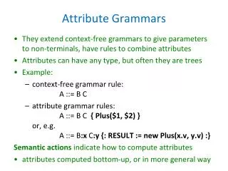
Functional Graphs • Definition: • A functional graph is a directed graph in which: • Nodes represent functions. • Incoming edges are parameters. • Outgoing edges represent functional values. • Edges represent data transmission among functions.
Example • Here we have three functions: • Constant function 2. • Constant function 3. • Binary function + (addition). • After some delay, the output value is 5. 2 3 + 5
Cycles in Functional Graphs • Can make sense only if the graph can achieve a steady state. • Example: • No steady state is achieved, because the output value keeps incrementing. 1 + ?
Example • A steady state is achieved. • If the "AND" were changed to a "NAND," no steady state. • Undecidable (halting problem) whether a steady state will ever occur. • We will assume that all functional graphs are acyclic. true and ?
Evaluation of Functional Graphs • First insert registers. • Then propagate values along the edges. • Register insertion: • Given edges E1 ... En from node A to nodes B1... Bn, • insert a register R: • one edge from A to R, and n • edges from R to B1 ... Bn.
Example • All registers initialized to some "undefined" value. • Top-most registers have no outgoing edges. B1 B1 gets converted to A B2 A B2 … … Bn Bn
Functional Value Propagation • Two algorithms: • Data Flow Analysis: repeated passes on the graph, evaluating functions whose inputs (registers) are defined. • Lazy Evaluation", performs a depth-first search, backwards on the edges.
Data Flow Algorithm While any top-most register is undefined { for each node N in the graph { if all inputs of N come from defined register then evaluate N; update N's output register } }
Lazy Evaluation for each top-most register R, { push (stack, R) } while stack not empty { current := top (stack); if current = undefined { computable := true; for each R in dependency (current), while computable { if R = undefined { computable := false; push (stack,R); } } if computable { compute_value(current); pop(stack); } } else pop (stack) }
Data Flow and Lazy Evaluation • Data Flow Analysis: • Starts at constants and propagates values forward. • No stack. Algorithm computes ALL values, needed or not.
Data Flow and Lazy Evaluation (cont’d) • Lazy evaluation: • Starts at the target nodes. • Chases dependencies backwards. • Evaluates functions ONLY if they are needed. • More storage expensive (stack), but faster.
Attribute Grammars • Associate constructs in an AST with segments of a functional graph. • It's a context-free grammar: • Each rule augmented with a set of axioms. • Axioms specify graph segments. • As AST is built (bottom-up); segments of the functional graph are "pasted" together.
Attribute Grammars (cont’d) • After completing AST (and graph), evaluate graph (data flow or lazy evaluation). • After graph evaluation, top-most graph register(s) (presumably) contain the output of the translation.
Definition An attribute grammar consists of: • A context-free grammar (structure of the parse tree) • A set of attributes ATT. • Each attribute "decorates" some node in the AST, later becomes a register in the functional graph. • A set of axioms defining relationships among attributes (nodes in the graph).
Example: Binary Numbers • String-to-tree transduction grammar: S → N => . → N . N => . N → N D => cat → D D → 0 => 0 D →1 => 1 • This grammar specifies "concrete" syntax. • Notice left recursion.
Abstract Syntax Tree Grammar • Use < ... > tree notation. S → <. N N> → <. N> N → <cat N D> → D D → 0 → 1 • This grammar (our choice for AG's) specifies "abstract" syntax.
Attributes • Two types: • Synthesized: pass information UP the tree. • Inherited: pass information DOWN the tree. • If tree is traversed recursively with (s1, … sn) ProcessNode(tree T, (i1,…,im)), • minherited attributes are parameters toProcessNode. • nsynthesized attributes are return values of ProcessNode.
Attributes (cont’d) For binary numbers, ATT = {value, length, exp}, where • value: decimal value of the binary number. • length: number of binary digits to the left of the right-most digit in the sub-tree. Used to generate negative exponents (fractional part). • exp: exponent (of 2), to be multiplied by the right-most binary digit in the subtree.
Attributes (cont’d) • Synthesized and inherited attributes specified by two subsets of ATT: • SATT = {value, length} • IATT = {exp} • Note: SATT and IATT are disjoint in this case. Not always.
Attributes Associated with Tree Nodes S: → PowerSet (SATT) I: → PowerSet (IATT) = { 0, 1, cat, . } (tree grammar vocabulary). S(0) = { value, length } S(1) = { value, length } S(cat) = { value, length } S(.) = { value } I(0) = { exp } I(1) = { exp } I(cat) = { exp } I(.) = { }
Example • Input: 10.1. • Convention: • Inherited attributes depicted on the LEFT. • Synthesized attributes depicted on the RIGHT. • Flow of information: top-down on left, bottom-up on right.
Tree Addressing Scheme Given a tree node T, with kids T1, ... Tn, a() denotes attribute "a" at node T, and a(i) denotes attribute "a" at the i’th child of node T (node Ti). • So, • v() is the "value" attribute at T • v(1) is the "value" attribute at T1. • v(2) is the "value" attribute at T2.
Rules for axiom specification. • Consider a production rule A → <r K1 ... Kn>. • Let r1, ..., rn be the roots of subtrees K1, ... , Kn. • Need one axiom per synthesized attribute at r (specify what goes up at root). • Need one axiom per inherited attribute at each kid ri(specify what goes to the kids). • Axioms are of the form a=f(w1, ..., wm), where each wi is either 3.1. inherited at r, 3.2. synthesized from ri, for some i. • Note: this doesn’t prevent cycles.
Attribute Grammar, Binary Numbers • Production rule S → <. N N>. • Need three axioms: • one for v at ".", • one for e at T1, • one for e at T2. • Axioms: value() = value(1) + value(2) exp(1) = 0 exp(2) = - length(2)
Notes • length attribute from kid 1 ignored. • length attribute from kid 2 is negated, sent down to e(2). Only use length to calculate negative exponents (fractional part, second kid). • length will start at 1, at the bottom of the tree. Will be incremented on the way up.
The Complete Attribute Grammar for Binary Numbers S -> <. N N> value() = value(1) + value(2) exp(1) = 0 exp(2) = - length(2) S -> <. N> value() = value(1) # no fraction; # copy value up. exp(1) = 0
The Complete Attribute Grammar for Binary Numbers (cont’d) N → <cat N D> value() = value(1) + value (2) # add two # values. length() = length(1) + 1 # increment # length up left. exp(1) = exp () + 1 # increment # exp down left. exp(2) = exp () # copy exp # down right. N → D # No axioms !
The Complete Attribute Grammar for Binary Numbers (cont’d) D → 0 value() = 0 # zero * 2exp. length() = 1 # initial length. D → 1 value() = 2 ** exp() # compute value. length() = 1 # initial length.
Example • Example, for input 10.1
Generation of Functional Graphs • Optional, see notes
Attribute Grammars Programming Language Principles Lecture 17 Prepared by Manuel E. Bermúdez, Ph.D. Associate Professor University of Florida